


The potential use of metabolomics approaches in nutritional studies has been discussed in recent reports (Whitfield et al. Reference Whitfield, German and Noble2004; Gibney et al. Reference Gibney, Walsh, Brennan, Roche, German and van Ommen2005). By analysing the metabolite content and concentration of a biofluid using NMR or liquid chromatography MS, a metabolic profile of a volunteer can be generated that provides a non-invasive ‘whole body snapshot’ (Holmes et al. Reference Holmes, Foxall and Nicholson1994; Lenz et al. Reference Lenz, Bright, Wilson, Morgan and Nash2003, Reference Lenz, Bright, Wilson, Hughes, Morrisson, Lindberg and Lockton2004; Kochhar et al. Reference Kochhar, Jacobs, Ramadan, Berruex, Fuerholz and Fay2006). Comparison of these snapshots before and after dietary intervention may highlight particular metabolites that respond (Solanky et al. Reference Solanky, Bailey, Beckwith-Hall, Davis, Bingham, Holmes, Nicholson and Cassidy2003, Reference Solanky, Bailey, Beckwith-Hall, Bingham, Davis, Holmes, Nicholson and Cassidy2005; Daykin et al. Reference Daykin, van Duynhoven, Groenewegen, Dachtler, van Amelsvoort and Mulder2005; Wang et al. Reference Wang, Tang, Nicholson, Hylands, Sampson and Holmes2005). This in turn may lead to potential biomarker identification and ultimately to a greater understanding of biochemical pathways.
There is some commonality in the type of data produced by post-genomic techniques. In general, it is highly multivariate: thousands of discrete data points are obtained from each sample examined, representing the action of many (known and unknown) variables within the system under study. Although the basic principles of the experimental techniques are well understood, the mathematical analysis of the data that come from such technologies has not been widely discussed in the nutritional literature. However, it is quite possible to misuse multivariate methods (Defernez & Kemsley, Reference Defernez and Kemsley1997), to the extent that meaningless conclusions are obtained; this is an issue that researchers need to be aware of when planning and conducting their work.
There is a collection of statistical techniques – the ‘chemometric’ approaches – that have become very popular for handling highly multivariate (or ‘high-dimensional’) data. One of the best-known of these is principal component analysis (PCA). PCA was first proposed over 100 years ago (Pearson, Reference Pearson1901) but for practical reasons was not widely used until the arrival of modern computing technology over the past two decades. PCA is a good method to use for data visualization and exploration. It compresses the data so that they are easier to examine graphically and in such a way that patterns may be revealed, which, although present, were obscured in the original data. Another data compression technique favoured by analytical chemists is partial least squares (PLS). Developed in the 1980s from the concept of iterative fitting (Wold et al. Reference Wold, Martens and Wold1982, Reference Wold, Ruhe, Wold and Dunn1984), PLS has been widely used in its basic regression form (Geladi & Kowalski, Reference Geladi and Kowalski1986).
In the present article, we present a case study comprising a set of high-resolution 1H NMR spectra of urine samples. These were obtained from a volunteer participating in a dietary intervention study designed to explore the role of dietary Cu in human metabolism. The data analysis challenge is to extract significant features from the spectra that show systematic differences between the ‘pre-’ and ‘post-intervention’ samples.
Various multivariate techniques are applied to the dataset and the advantages and disadvantages of each are discussed, along with some of the pitfalls that may be encountered in the analysis of high-dimensional data. We will show that neither PCA nor PLS are sensitive enough when the most relevant spectral information is concentrated in a few very small peaks, even a single peak, set against the ‘background’ of many other larger peaks varying in ways unconnected with the grouping of interest. An alternative to the whole-spectrum approach in these circumstances is feature subset selection (Leardi et al. Reference Leardi, Boggia and Terrile1992; Yoshida et al. Reference Yoshida, Leardi, Funatsu and Varmuza2001; Tapp et al. Reference Tapp, Defernez and Kemsley2003). Genetic algorithms (GA) are effective at selecting variables from large datasets and in the present work we have implemented a GA to conduct a search for small subsets of peaks that are the most useful discriminators.
The case study
Six healthy male subjects aged 34–57 (mean 39) years were recruited to a dietary intervention study investigating human Cu metabolism (Harvey et al. Reference Harvey, Dainty, Hollands, Bull, Beattie, Venelinov, Hoogewerff, Davies and Fairweather-Tait2005). A 10 ml screening blood sample was taken to exclude volunteers whose biochemical and haematological indices fell outside the normal range. Other exclusion criteria included taking medication or nutritional supplements and smoking. The aims and procedures of the study were explained to the volunteers during a visit to the Human Nutrition Unit at the Institute of Food Research, and written informed consent was obtained. The Norwich District Ethics Committee approved the protocol and the study was conducted in accordance with the Declaration of Helsinki 1975, as revised in 1983. In the present article, we primarily discuss the data from a single volunteer, as an example dataset with which to illustrate the multivariate techniques. Data from a second volunteer are introduced as a fully independent test set, with which to illustrate the concept of external validation in multivariate analysis. All other results will be reported in a separate article, in which the emphasis will be on the results of the study from a biochemical perspective.
The study consisted of three experimental periods, and all subjects were free-living throughout. Collection of urine samples for metabolomic analysis formed only part of the experimental protocol (see Harvey et al. Reference Harvey, Dainty, Hollands, Bull, Beattie, Venelinov, Hoogewerff, Davies and Fairweather-Tait2005). During the first experimental period (EP1), complete 24 h urine collections were made over 8 consecutive days. During the second experimental period (EP2), a minimum of 4 weeks later, the subjects collected a further eight consecutive 24 h urine samples. Volunteers kept a record of all food and beverages consumed for 2 d before and days 1–5 of EP2 urine collections. Following EP2, volunteers consumed a daily Cu supplement containing 6 mg Cu for 6 weeks and then collected 24 h urine samples for 8 consecutive days (EP3). During EP3, volunteers were asked to consume the same food and beverages on the 2 d before and days 1–5 of urine collection as those recorded for EP2.
Spectral acquisition
Urine samples were prepared for NMR analysis by mixing 500 μl urine with 200 μl 0.2 m-phosphate buffer (pH 7.4) in D2O containing 1 mm-sodium 3-(trimethylsilyl)-propionate-d 4 as a chemical shift reference. Samples were shaken and 600 μl were transferred into a 5 mm NMR tube for spectral acquisition. 1H NMR spectra were recorded at 600.13 MHz on an Avance spectrometer (Bruker BioSpin, Rhe stetten, Germany) equipped with an auto-sampler and a BBI probe fitted with z gradients. After locking on the D2O signal and carrying out automatic gradient shimming, spectra were acquired on non-spinning samples at 300°K using the nuclear Overhauser effect spectroscopy-presaturation sequence (RD – 90° pulse – t 1 – 90° – t m – 90° – ACQ) with relaxation delay (RD) 2 s, 90° pulse 10.6 μs, t 1 4 μs, mixing time (t m) 150 ms, acquisition time (ACQ) 1.95 s. The water signal was suppressed by applying low power irradiation at the water frequency during RD and t m. For each sample, 128 transients were acquired into 32 K time domain points with the spectral width set to 14 ppm. The time domain signals were Fourier transformed with a 1 Hz exponential line broadening factor, zero filled to give spectra with 32 K real points and automatically phase corrected.
Data pre-processing
Manual baseline correction was performed (usually only the first two terms of a fifth order polynomial correction were used). Spectra were aligned along the ‘chemical shift’ axis (see later) by setting the trimethylsilyl-propionate-d 4 signal to 0 ppm. This sets all spectra onto a common horizontal scale across most of the spectral range. However, in certain regions of the NMR spectrum, the registration issue is too complicated to be solved by simple sideways shifting. For instance, in the spectra discussed here, the two doublets arising from citrate vary somewhat in position from sample to sample. This type of problem is acknowledged in the literature and various methods have been proposed to deal with it. A common pre-processing approach is to de-resolve the dataset by ‘binning’ (Holmes et al. Reference Holmes, Foxall and Nicholson1994) – dividing the horizontal axis into (equal or unequal) regions and calculating a sum of the spectral intensity in each. Broader bins can be defined to cover, say, each of the citrate doublets and so the resulting ‘binned’ data are less sensitive to the registration problem (Wang et al. Reference Wang, Tang, Nicholson, Hylands, Sampson and Holmes2005). In the past, binning has been standard practice in dealing with NMR data, not least because the binned spectra contain far fewer data points than the original data, substantially reducing the computational load in any subsequent multivariate analysis. The penalty, however, is considerable loss of spectral resolution. Minor but important signals may be included in the same bin as major but non-significant signals. At best, this complicates the interpretation; at worst, important information may be obscured and overlooked. Given the continuing advances in microprocessor performance, we no longer believe that binning is necessary on the grounds of computational load. Instead, we have elected, as others are now doing (Cloarec et al. Reference Cloarec, Dumas, Trygg, Craig, Barton, Lindon, Nicholson and Holmes2005), to make use of all the spectral resolution as acquired, whilst acknowledging that a few regions of the spectrum will suffer from poor peak alignment.
The files containing the resulting spectra were converted to JCAMP-6 format text files and imported to Matlab®, version 7 (The Mathworks, Inc., Natick, MA, USA). All subsequent algorithm development and data analysis was carried out within the Matlab environment. Further pre-processing steps are described later, along with the descriptions of the multivariate methods employed.
High-resolution NMR spectra
High resolution 1H NMR data were recorded from the 24 h urine specimens from each volunteer, in random order. An NMR spectrum comprises a horizontal axis recording the ‘chemical shift’ values, with a vertical axis that records the signal intensity at each of many thousands of those chemical shifts. For any given metabolite every distinct hydrogen atom or group of equivalent hydrogen atoms (for instance, the three hydrogens in a methyl group) gives rise to a NMR signal at a chemical shift that is characteristic of the chemical environment of that hydrogen. The signal can be a singlet or a multiplet: the multiplet structure arises from interactions with neighbouring hydrogen atoms and generally the multiplicity increases with the number of ‘near-neighbour’ hydrogens. The intensity of the NMR signal (strictly, the area under the signal) is directly proportional to the concentration of the parent molecule in the biofluid mixture. This is the basis for the use of NMR as an analytical technique (Günther, Reference Günther1995) and is also fundamentally the reason why data analysis based upon linear algebra methods is so effective. Under the conditions of our experiment a few types of hydrogen atom, such as those bonded to oxygen or to some nitrogen atoms, exchange with hydrogen atoms of water and do not give a signal. However, the vast majority of metabolites contain hydrogen atoms linked to carbon and all of these hydrogens give observable signals. Thus, most metabolites can be detected if their concentrations are sufficiently high. The main caveat is that all metabolites present in the biofluid (possibly several thousand in urine) are detected simultaneously; because the chemical shift range for hydrogen is rather limited there is inevitably some signal overlap. The water signal itself is massive compared with signals of the metabolites and has to be suppressed in order to measure those much weaker signals.
Each spectrum usually comprises a very large number of discrete intensities – in the case of the present study approximately 32 000. Due to this very large number, ‘joining the dots’ in a graphical display gives a series of peaks of different heights, with the appearance of a smooth, continuous trace. Spectra are relatively easy for the human eye to assess; patterns of peaks and troughs quickly become familiar and an experienced spectroscopist can often recognize the spectrum of a particular chemical compound immediately. In addition, a vast amount of work exists in the literature on the assignation of spectral bands to particular chemical entities, so that in some cases quite detailed elucidation of the composition of the specimen is immediately possible (Fan, Reference Fan1996; Lindon et al. Reference Lindon, Nicholson and Everett1999).
All twenty-four spectra obtained from one individual's urine specimens are shown in Fig. 1(a) (the spectra are offset vertically, for clarity). Although some sections of the spectrum can be discarded as ‘baseline’ (i.e. containing no information other than noise), around 22 000 intensity values contain spectral information (peaks) in some or all of the recordings and these were retained for subsequent data processing. There are several points to note here. The size of spectral peaks arising from individual compounds varies over orders of magnitude (compare the large peaks at around chemical shifts 3–4 ppm with those in the region, say, 7–8 ppm). In fact, there are many features that can only just be discerned as tiny bumps along the baseline on this figure, but simply by expanding the scale these are revealed as clear, well-resolved spectral bands. Fig. 1(b) shows an expansion of the region 2–2.8 ppm (comprising 2000 data points), again stacked vertically. This gives a graphic impression of the sensitivity of the NMR method.
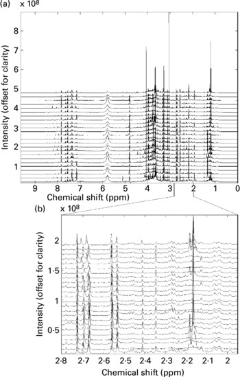
Fig. 1 (a) A set of high-resolution NMR spectra collected from twenty-four urine samples from a single volunteer. Spectra are shown offset for clarity; (b) an expansion of a region of the data shown in Fig. 1a. Spectra are shown offset for clarity.
It also illustrates the substantial variation within a single volunteer's measurements: note, for instance, the changing patterns of peaks in the region around 2.1–2.2 ppm. Four singlets with chemical shifts between 2.15 and 2.18 ppm that are seen in several of this volunteer's traces can be assigned to metabolites of paracetamol (Bales et al. Reference Bales, Sadler, Nicholson and Timbrell1984). Signals from ethanol and metabolites of common analgesics are commonly found in a proportion of urine spectra in studies where no dietary restrictions are imposed. The signals need to be recognized, but can then generally be disregarded.
These figures illustrate the data visualization problem in NMR experiments. Even from a modest collection of spectra (twenty-four spectra in total), the number of data points (and spectral peaks) that need to be examined is very large indeed. Whereas some differences between spectra are immediately obvious, others are much more subtle and, moreover, it is not readily apparent which regions of the spectrum contain the most relevant information. In this case study, we will concentrate on identifying systematic and meaningful differences between the ‘pre-’ and ‘post-intervention’ samples collected from a single volunteer – the challenge is to isolate these from the large background of within-individual variance.
Multivariate techniques
A number of key concepts underpin the effective use of multivariate statistical methods in the analysis of high-dimensional data. Consider first of all a hypothetical, simplified spectrum that comprises measured intensities at just three chemical shift values. Since there are three ‘variables’, each of which is measured independently of the others, the data are described as three-dimensional (the dimension simply means the number of independent variables). Consider now a set of twenty-four such measurements, as illustrated in Fig. 2(a). This is the standard way in which spectra are represented, but this very small dataset could equivalently be plotted as twenty-four points on a three-dimensional coordinate system, with axes given as ‘chemical shift 1’, ‘chemical shift 2’ and ‘chemical shift 3’ (Fig. 2(b)). The number of points recorded on this plot equals the total number of spectra.

Fig. 2 (a) A set of simulated ‘spectra’ consisting of only three variables (at three chemical shift values); (b) illustration of the concept of rigid data rotation, as implemented in principal component analysis and partial least square data compressions.
Of course, real NMR spectra comprise intensities measured at thousands of chemical shifts: the case-study dataset under discussion contains 22 000. If it were possible to depict 22 000 axes in some way, then each spectrum could be plotted as a single point in this space, mimicking the simplified three-dimensional example. In practice, plots in two and three dimensions are straightforward, but representing 22 000 dimensions graphically is clearly hopeless.
Central to multivariate statistics are the ideas of variance and covariance. Covariance measures how much two supposedly unrelated variables vary together: if two variables have no association whatever then their covariance is zero, meaning that as one variable changes the other pays no heed. Variance is a special case of covariance that quantifies the variation in just a single variable. PCA and PLS are based on the calculation of a covariance matrix (or, in related alternative definitions, a correlation matrix; this is discussed further later). This is a square table displaying how all the possible combinations of pairs of variables are associated with one another; the diagonal of the matrix contains the variances of each variable. The covariance matrix directly summarizes the information content of the original dataset, although hardly in a concise form; in our NMR data, for instance, the covariance matrix is 22 000 rows by 22 000 columns and so contains >400 million elements. Again, this represents no problem from the mathematical perspective, but hints at the data handling and visualization challenges; it is impossible to make sense of this quantity of information without some systematic help.
Principal component analysis
The goal of PCA is to provide that help. In PCA, the aim is to generate a new set of variables that are simple linear combinations of the original data. Graphically, this corresponds to rotating the original variable axes onto a new coordinate system. In the three-variable example, this can be readily visualized: the plotted points are left dangling in space while the axes are rotated about the origin (see Fig. 2(b)). The original data values are replaced by ‘scores’: these are projections of each point onto the new axes. In addition to the scores, we obtain as an output a series of lists of the relative weights of the original variables that must be blended together to form each new score. These lists are called principal component (PC) ‘loadings’; graphically, the loadings define the rotated axes relative to the original axes. The new coordinate system has lost the transparent interpretation of the original axes, but this turns out to be a price worth paying.
There are rules to guide the selection of the new axes. First, they must be at right-angles (orthogonal) to one another, just as the original axes were mutually orthogonal. Second, the new axes are chosen so that the scores along each axis are uncorrelated with those along any other. This is central, since in the original data, the values along any one axis typically were correlated to some extent with those along other axes. The axis rotation translates mathematically to transforming the original covariance matrix into a diagonal matrix; in other words, a matrix relying solely on variances of the scores. There are standard mathematical techniques for performing this operation.
So, how does this procedure help? PC scores are ranked according to the magnitude of their variance and, typically, the variances of the first two or three scores will express well over half the total variance of the original dataset. If this is the case, then the remaining scores can be ignored on the grounds that they contribute little to the data variability. This is an example of what chemometricians call ‘data compression’ or ‘dimension reduction’ – reducing the number of variables from, say, 22 000 to just two, yet retaining most of the information. So PCA is about describing the data, originally expressed by large numbers of manifest variables, in terms of a handful of latent (underlying) variables selected to encompass virtually all of the original information content. PCA is especially useful when much of the data are ‘the same’, which in the context of NMR means that the spectra of many samples are broadly similar; such data are described as multicollinear or highly redundant. It is also useful when the number of variables (for instance, the number of intensity values in each NMR spectrum) greatly exceeds the number of observations (the total number of spectra).
Whereas 22 000 dimensions would be impossible to plot, it is simple to plot two and so a typical PCA output is a display of the first v. second PC scores. Fig. 3(a) shows the first v. second scores obtained from PCA applied to the set of twenty-four NMR spectra; recall that each point on this plot represents a single spectrum. In carrying out PCA, the hope is that patterns or groups of points will emerge in the scores plot, reflecting underlying structure present but obscured in the original data. When this is the case, then a mathematical ‘audit trail’ can allow us to trace back from points in the PC plot, via the loadings, to features in the original spectra. Unfortunately, we find no such interesting patterns in the present example; the points representing spectra from the two groups of interest are substantially overlaid.

Fig. 3 (a) Principal component (PC) scores of the raw NMR dataset; (b) partial least squares (PLS) scores of the raw NMR data. (c) PLS scores of ‘noise’ with the same dimensions as the NMR data. (d) Cross-validated PLS scores of the NMR data. For plots (a), (b) and (d), ○, ‘pre-intervention’ samples; ■, ‘post-intervention’ samples.
Now, PCA scores represent successively maximized sources of variance in the data, but this does not mean that the first two PCs are necessarily the most interesting. In our example, they might be exposing variation in the data due to confounding factors (such as age or diet in general), rather than variation due directly to the Cu supplementation. The lesson is to explore beyond the first two PCs, perhaps plotting various combinations including the third or even the fourth. However, in our present work, neither the third nor fourth PC showed any interesting clustering either. In addition, there is a slight ‘health warning’ associated with lower ranking PC; these are associated with decreasing variance and increasing instability. In our example, the variances associated with the first six PC are respectively 28 %, 22 %, 17 %, 14 %, 6 % and 3 %. When the variance of a PC is of the order of 1/n, where n is the number of observations, then that PC could represent the influence of a single observation only. As a rule of thumb, it is unwise to place much reliance on such low-ranking PC.
Partial least squares
One important feature (and limitation) of PCA is that it operates solely on the matrix of experimental data and does not take into account any additional information that may be associated with each measurement. For instance, in the present case the sample provenance information – sixteen spectra are designated ‘pre-’ and eight ‘post-intervention’ – is not utilized in the PCA transformation. A related approach, PLS, attempts to plug this gap. More fully, PLS stands for partial least squares projection onto latent structures. Rather than simply exposing the dominating contributions of the experimental data, PLS requires a second matrix of information relating to each sample. In statistical language, this is a matrix of dependent variable(s). It uses this additional information in an attempt to reduce the influence of irrelevant data points on the data compression.
Again thinking geometrically, PLS first constructs a single new axis whose direction is dictated by maximizing the covariance between the observed and the dependent variables. With the best possible new axis determined, the data are then projected onto it to yield corresponding scores. The projected part of the data is subtracted from the complete dataset and the process repeated on the residual data to find the next most relevant axis, and so on.
A typical PLS scores plot will display the first few scores plotted against one another, analogous to the kind of plots produced in PCA. The interpretation is much the same, only it is now somewhat more likely that the scores plot will reveal patterns relating to the question of interest. However, PLS has not automatically usurped PCA for a very important reason: compared with PCA, PLS is prone to ‘overfitting’. The outcome of overfitting can be seriously misleading, with the added difficulty that the problem is not always obvious. Consider Fig. 3(b), which shows the first two PLS scores calculated from our twenty-four NMR spectra, using a ‘dummy’ dependent variable to encode the ‘pre’ and ‘post-intervention’ category associated with each spectrum. On first inspection, this appears to hold promise; there is clearly some division of the points into the two groups of interest. Is PLS able to detect a systematic difference between the groups? Unfortunately not – it turns out that this misleading plot is the result of an overfit data compression, as we will now see.
Overfitting can arise in PLS when there are very many more variables than samples. In fact, overfitting is an ever-present danger in any analysis of high-dimensional data: it is an unavoidable hazard of trying to extract reliable information from massively under-determined experimental data – in post-genomic measurements, there are almost always many, many more variables than independent samples. When the data are very high-dimensional and the experiment as a whole is under-determined (as in the case of the NMR spectra: 22 000≫24), then it is highly likely that there will be one or more variables with values that provide accidental correlation with the dependent variable. As an example, consider twenty-four ‘spectra’, each containing nothing but 22 000 data points of noise. We can allocate these at random into two arbitrary groups. Reassuringly, PCA conducted on this dataset will discover no signature by which the different ‘spectra’ can be classified. However, Fig. 3(c) shows the outcome of applying PLS to the same ‘toy’ example. This apparently clear discrimination was extracted from a dataset comprising random noise allocated to meaningless groups!
Real life data are unlikely to behave in quite such an extreme fashion as the simulated noise, but it is entirely possible to generate outcomes similar to that of Fig. 3(b), which appear plausible but are in fact overfit. A common and straightforward way to test for overfitting is to systematically discard each spectrum from the dataset one at a time, use the retained data to develop a model and then apply this model to the discarded item to obtain a ‘prediction’ (of scores or group assignment, say). Only the scores from the cross-validation items are reported or plotted in a PLS scores plot. This is called leave-one-out cross-validation and is one of a variety of validation strategies in multivariate analysis. The idea is that if there is genuinely underlying structure in the data, then the PLS compression will be stable enough to withstand the successive omission of individual observations, and the scores of the cross-validation items will still be able to reveal the groupings or patterns of interest. PLS was applied in cross-validated form to the NMR data. The scores plot obtained is shown in Fig. 3(d). We see that the apparent discrimination depicted in Fig. 3(b) is not maintained under cross-validation and must therefore be disregarded.
Data pre-processing: scaling, filtering and normalization
Scaling
In the most usual definitions of PCA and PLS, the loadings are eigenvectors of a covariance matrix. Earlier, we have described the application of these forms of PCA and PLS directly to raw NMR spectra. However, in addition to other forms of PCA and PLS, there also exists a range of data pre-treatments, which are commonly used in conjunction with multivariate analysis of spectral data. We will discuss some of the most commonly encountered approaches here and illustrate their effects using the data from our case study.
Both PCA and PLS can be defined slightly differently, such that the loadings are instead eigenvectors of a correlation matrix. Numerically, this is equivalent to ‘standardizing’ the dataset before proceeding with covariance-method data compression. Standardization involves scaling the data (by subtracting the mean and dividing by the standard deviation) so that each variable has zero mean and unity variance. An effect of standardization in the context of data compression is to prevent variables with very large variances (and covariances) from dominating the selection of the compressed axes. Since NMR spectra can contain peaks with order of magnitude intensity differences, the variance of the largest peak in a dataset can be vastly greater than that of the smallest (even though their CV may be similar). It is therefore common practice to use scaling of some kind when analysing NMR data. An alternative to standardization is pareto-scaling, in which each variable is divided by the square root of its standard deviation. The use of these and other scaling methods (e.g. range scaling, log transformations) in metabolomics has been discussed (van den Berg et al. Reference van den Berg, Hoefsloot, Westerhuis, Smilde and van der Werf2006). A disadvantage of scaling is that standardized spectral data no longer look like spectra (Fig. 4(a) shows the same data as in Fig. 1(a), but now standardized), and neither do products of the data compression (i.e. the loadings). ‘Inverse variance-scaling’ of loading vectors has been proposed as a means of assisting visualization and some authors have suggested additional graphical aids to interpretation (Cloarec et al. Reference Cloarec, Dumas, Trygg, Craig, Barton, Lindon, Nicholson and Holmes2005).

Fig. 4 Illustrating data pre-processing. (a) ‘Standardized’ spectra (the same data as shown in Fig. 1(a), but here it has been mean-centred and scaled to unit variance); (b) threshold filtering: the points representd the variables retained.
Filtering
The central difficulties in high-dimensional data analysis arise from the great disparity between the number of observations and the number of variables, so an obvious approach is to reduce this mismatch in some way. As discussed earlier, binning is a commonly used means of reducing the dataset size, but will not be employed in our present work as we want to be able to exploit the high spectral resolution of our data.
Some reduction of variables can generally be made by using an expert's judgement to discard portions of the spectrum known to contain no useful information (indeed, in our example, we were able to immediately reduce the data from 32 000-variate to 22 000-variate by discarding approximately 10 000 variables that contained noise only). A straightforward extension of this approach is to pass the data through a threshold filter, retaining only those variables that exceed some pre-defined threshold. Using a filter set at just above the level of the ‘chemical noise’, we were able to further reduce our dataset to around approximately 15 000 points (Fig. 4(b)).
Normalization
Another type of pre-treatment that is often encountered in the analysis of spectral data is normalization. This is used to scale entire spectra simultaneously (rather than individual variables separately); again, there are different kinds of normalization and the choice of transformation is related to considerations of spectral acquisition and experimental protocol. For example, in our case study, the total concentration of metabolites in each urine sample is not known, nor can it be easily controlled. Consequently, the variance in the raw spectral data may be dominated by variability in total compound concentration, which is not as interesting as relative concentration of individual metabolites. To mitigate this effect, we can use ‘area-normalization’ – scaling the data so that the integrated spectral intensity is set to unity, without altering the relative heights of the peaks within each spectrum. The rationale behind this and some other less common normalization methods has been examined (Craig et al. Reference Craig, Cloarec, Holmes, Nicholson and Lindon2006) and a more sophisticated approach has been proposed (Dieterle et al. Reference Dieterle, Ross, Schlotterbeck and Senn2006) to deal with some anomalies that can arise.
The various kinds of pre-processing (scaling, filtering, normalization) can be applied individually, or in combination and in different orders. In the interests of conciseness, we will not attempt an exhaustive comparison of all possible combinations – given the range of different approaches and ‘variations on a theme’, this is really rather large. As an illustration, however, Fig. 5 shows how the outcome of cross-validated PLS on our example dataset is affected by selected pre-treatment combinations. The benefits of pre-processing in this case are clear. Specifically, Fig. 5(d) shows the outcome of cross-validated PLS after three pre-treatments: (i) normalization to unity integrated spectral intensity; followed by (ii) threshold filtering to the variables shown in Fig. 4(b); finally (iii) variance-scaling. There is clearly now some distinction between the two groups of interest (compare it with Fig. 3(d)). In this instance, variance-scaling appears to have produced the greatest benefit – this hints that minor peaks are important in differentiating the groups, but were unable sufficiently to influence the PLS transformation without variance-scaling.

Fig. 5 Cross-validated partial least squares (PLS) scores shown after various combinations of pre-treatment. (a) Filtering only; (b) filtering and standardization; (c) ‘area-normalization’ and filtering; (d) area-normalization, filtering and standardization. ○, ‘pre-intervention’ samples; ■, ‘post-intervention’ samples.
Feature subset selection
PCA and PLS are widely used techniques that can perform well in many different applications. However, sometimes the most important and relevant information is concentrated in spectral peaks that are too small and/or too few to influence the data compression sufficiently. An alternative to the whole-spectrum approach in these circumstances is feature subset selection. This involves searching for small subsets of peaks or data points that are the most useful, as judged by some appropriate criterion. Variable selection algorithms have long been used as precursors to multivariate analysis of spectroscopic data. There are two main challenges with this approach. First, when the total number of peaks to choose from is very large, then the number of possible subsets becomes astronomical. For instance, if the data contains approximately 15 000 variables, and if we want to search for even a small subset comprising, say, just four, then there are approximately 1015 possible combinations! However, GA have been found to be effective at selecting variables from high-dimensional datasets (see Leardi et al. Reference Leardi, Boggia and Terrile1992).
GA are a particular class of evolutionary algorithms; numerical optimization procedures that employ biologically inspired processes such as mutation and selection. In a GA, a population comprising randomly generated trial solutions (‘chromosomes’) is evaluated to yield a ‘fitness’. Next, a new generation of solutions is created through reproduction, with the fitness function determining how likely any individual chromosome is to reproduce. The process is iterated for a number of generations, until an acceptable solution has evolved.
In the present work, we have implemented a GA to search for small subsets of peaks, which collectively distinguish the ‘pre-’ and ‘post-intervention’ spectra. In this context, each chromosome identifies a small subset of peaks (i.e. chemical shift values) and the fitness criterion is success rate in two-group cross-validated linear discriminant analysis (LDA; this is a well-known technique for treating classification-type problems in multivariate data (see for example Seber, Reference Seber1984)). The dataset passed to the GA had been area-normalized and filtered (i.e. the same pre-treatments that had been applied to the data in producing the PLS plots in Fig. 5(d); note that variance-scaling is implicit in the form of LDA used, which measures ‘distances’ between spectra using the Mahalanobis metric).
A schematic illustrating the GA procedure is shown in Fig. 6. The criterion for termination of GA evolution was attainment of a 100 % classification success rate, which was generally achieved in less than ten generations. We searched for a subset size of four, with an initial population size of 4000 chromosomes. The brief outline given here indicates that in implementing a GA, the user is required to set rather a lot of parameters (including the mutation rate, subset size, number of chromosomes, fitness and convergence criteria), all of which will affect how the GA performs. Some of these largely affect the rate at which the GA converges; our choices for these parameter values have been based upon experience. The interested reader can download our GA routine (as a Matlab m-file from www.metabolomics-nrp.org.uk/publications).

Fig. 6 Simple schematic showing the main steps involved in a genetic algorithm (GA) for feature selection in NMR data.
The complete GA routine (‘epoch’) was carried out repeatedly (1000 repeats), because the random nature of the initial chromosomes, and the various processes during the GA, affect the outcome of any single epoch. The best solution(s) from each epoch were retained. At this juncture we need to consider another ‘health warning’, concerning the second challenge of the feature selection approach. This is again related to the inherently under-determined nature of experiments involving high-dimensional data. When there are very large numbers of peaks to choose from, and relatively very few spectra, then it is inevitable that some data points (even noise along the spectral baseline) will by chance fit the structure being sought – and an efficient GA will seek these out and identify them. The greater the subset size sought, the more easily the GA finds it to overfit and this needs to be kept in mind when setting this parameter. Even cross-validation is insufficient protection against this particular form of overfitting, when there is such a disparity between the dimensions of the data and the number of observations.
Alternative validation approaches (e.g. partitioning into training, tuning and independent test sets) are possible if there are sufficient measurements – in the present case study, however, the small size of the ‘post-intervention’ group makes these approaches awkward within one volunteer's data. However, in the present study, spectra from additional volunteers were available. If the peaks and regions identified by the GA are found to be useful discriminators in these fully external ‘validation’ datasets, then this would suggest that the GA has highlighted variables that are genuinely related to the question being addressed (rather than spurious variables that happened fortuitously to fit the structure being sought in the training data). We will consider this further later, but first let us discuss the results obtained directly from executing the GA.
From the 1000 epochs, over 12 000 unique solutions were obtained, all of which gave a success rate of 100 % in cross-validated LDA (recall that each solution is a subset of variables at four different chemical shift values). It may seem surprising that so many equivalent solutions exist, but in fact this high degree of redundancy is, in the present case study, a manifestation of overfitting – with so many variables to choose from (>15 000), it is to be expected that there are many combinations of four variables, which by chance alone will collectively allow such small sample group sizes (sixteen and eight respectively) to be discriminated.
The purpose of executing multiple GA epochs with randomized initial chromosomes is to establish whether there are any variables with a greater tendency to persist in each population – these are likely to be the best discriminators. Fig. 7 presents a histogram showing the frequency of occurrence of each variable across all the solutions (along with the average NMR spectrum). The histogram can be considered as a ‘pseudo-loading’, with spectral-like features: the ‘peaks’ indicate the most consistently effective discriminators. However, the ‘noise’ along the bottom of the histogram shows that subsets can be found that include virtually any data point in the spectrum! Even if we consider only the histogram ‘peaks’, there are rather a lot of data points (or regions) that appear to be useful. If we examine the average spectrum (shown in the upper half of the figure) plotted on the same axis, we find that the majority of the histogram maxima correspond to relatively small spectral signals. Although at this stage we cannot be confident that the GA has identified genuinely important spectral peaks, it is at least consistent with the outcome of the cross-validated PLS analyses described earlier, which clearly benefited from variance-scaling.

Fig. 7 Histogram showing relative frequency of occurrence of each data point within the 12000 best solutions obtained from the genetic algorithm (GA) repeats and, on the same horizontal scale, the mean of the raw NMR spectra.
The region of the spectrum identified as perhaps the most useful corresponds to chemical shifts in the range 0.7–1.1 ppm. These are very small signals in the raw data; an expansion of approximately 700 data points taken from all twenty-four spectra in this region is shown in Fig. 8. Underneath is a corresponding expansion of the GA histogram. The largest ‘bands’ are peak-picked and labelled with the corresponding chemical shifts. Detailed inspection of the chromosomes showed that the large majority of solutions contained variables taken from across different bands (as opposed to several from within one band). Within this spectral region alone, many combinations of only three variables taken from across any of the main histogram bands will produce complete separation of the groups. This can be seen graphically by plotting the variables against one another. Fig. 9(a) shows the standardized data from, as an example, chemical shifts 0.848 ppm, 0.861 ppm and 0.755 ppm, plotted against one another. The two groups are clearly linearly separable; however, we emphasize once more that this outcome must be treated cautiously – in view of the unavoidable potential for overfitting, it is a meaningless finding unless it can be externally validated by some means.

Fig. 8 An expansion of a spectral region identified as important by the genetic algorithm feature selection. Spectra are shown offset for clarity. The lower part of the figure shows an expansion of the histogram in the same region. Main ‘features’ in the histogram are marked with the corresponding chemical shift.

Fig. 9 Data from three variables only (chemical shifts 0.848 ppm, 0.861 ppm and 0.755 ppm) taken from area-normalized and standardized datasets from the ‘training set’ volunteer (a), and additional volunteers (b)–(f). LDA, linear discriminant analysis; ICV, internal cross validation; Hypothesis H0a, the trivariate data for each volunteer contain no group structure; Hypothesis H0b, all subsets of three peaks have the same discriminatory performance. For details, see Feature subset selection.
Thus far, we have discussed the data obtained from a single volunteer's samples, as a concise example with which to illustrate the multivariate methods. We now consider briefly the data from the remaining five volunteers – a total of 120 further NMR spectra. These data have not been used in any of the modelling work and so constitute entirely independent data. Fig. 9(b)–(f) show the data from the same three chemical shifts as in Fig. 9(a), plotted for each of the remaining five volunteers. Each volunteer's dataset was pre-processed in the same way (area-normalized and standardized). For all five further datasets, the plotted points show evidence of discrimination between the dietary intervention groups. Cross-validated LDA was carried out for each volunteer using just these three data points. The success rate obtained is marked on each plot. For volunteers (b)–(f), we also test the following hypotheses: H0a – the trivariate data for each volunteer contain no group structure; H0b – all subsets of three peaks have the same discriminatory performance. In both cases, the test statistic used was the cross-validated success rate, the empirical distributions of which are obtained by permutation resampling (10 000 resamples in each case). Permutation tests are a subset of non-parametric statistics (see for example, Westfall & Young, Reference Westfall and Young1993, or http://en.wikipedia.org/wiki/Resampling_(statistics)#Permutation_tests). The P values for H0a and H0b are marked on the figure. We can conclude that there is strong evidence that these spectral features genuinely play a role in distinguishing the pre- and post-intervention groups.
Notice that different rotations of the axes are required in order to best highlight the distinction between groups. This indicates that multivariate models developed using one individuals' data will not generalize to data from a different individual, which is why the LDA modelling discussed earlier was carried out for each individual separately. The reason for this is straightforward; there is very large between-volunteer variance. In the present article we simply make this observation. A full discussion of inter-individual variation in NMR spectra of urine samples will form the subject of a separate publication.
External validation can additionally take the form of expert assessment – what are the peaks identified by the GA and are the findings biochemically plausible? Returning once more to Fig. 8, one of the most distinct features is the doublet at 0.75 ppm (splitting 6.8 Hz). This doublet can be seen in every one of the bottom sixteen traces (corresponding to pre-dose periods EP1 and EP2) in Fig. 8, but only in one of the top eight traces (post-dose period EP3). Additional two-dimensional NMR experiments on one of the afore-mentioned samples showed that the doublet at 0.75 ppm was associated with two other signals, at 0.88 and 2.18 ppm (the latter being responsible for the 6.8 Hz splitting). It has not been possible to identify the compound itself from available databases but it is likely that the two signals at 0.75 and 0.88 ppm are from the two methyl groups of an isopropyl unit with the methine hydrogen of the fragment giving the signal at 2.18 ppm. The non-equivalence of the two methyl groups indicates that the isopropyl group is linked (or is in close proximity) to a chiral centre.
In a final comparison of methods, PCA and cross-validated PLS were applied to the ~0.7–1.1 ppm region (area-normalized, filtered, variance-scaled data). The PC and PLS scores plots are given respectively in Fig. 10(a), (b). This again illustrates the difference in power between the techniques. PCA highlights only slightly the difference between the two groups in the first two dimensions; clearly, other variances such as the very obvious intensity differences at around 0.87 ppm, which are unrelated to the ‘pre-‘ and ‘post-intervention’ groups, are dominating the data compression. PLS, in contrast, is specifically seeking the grouping of interest and is able to promote this source of variance into the first two PLS dimensions.

Fig. 10 Scores plots obtained from applying (a) principal component (PC) and (b) partial least squares (PLS) to the spectral region shown in Fig. 6. ○, ‘pre-intervention’ samples; ■, ‘post-intervention’ samples. (c) Plots of the first and second PLS loadings obtained from the spectral region of Fig. 9, on the same horizontal axis as the mean spectra of the ‘pre-’ and ‘post-intervention’ groups. Loadings are shown ‘inverse-variance-scaled’.
The separation between samples in the PLS scores plot is ‘explained’ by the two PLS loadings, which are shown in Fig. 10(c), along with the mean spectra from the pre- and post-intervention periods for comparison. (Recall that scores are weighted sums of the original data, with the loadings supplying the weights; plots of the loadings therefore show the relative importance of each original variable to each PLS dimension.) Fig. 10(b) shows that the pre-intervention group tends to have more positive scores on PLS axes 1 and 2; post-intervention samples tend to have more negative scores on both axes. Loadings 1 and 2 in Fig. 10(c) both show three prominent doublets (approximately 0.75, approximately 0.91 and particularly approximately 0.88 ppm), all with positive signs, which indicates that the compounds responsible for these signals have increased levels in the pre-intervention group. The difference in the 0.75 ppm doublet is apparent from the two mean spectra (and Fig. 8), but the loading highlights the involvement of the other two doublets much more clearly than the mean spectra and provides independent corroboration that a single compound is responsible for the doublets at 0.75 and 0.88 ppm.
It would be premature to conclude that changes in the level of this compound, or the other compounds picked out by the GA, are a direct consequence of the Cu supplementation. Stronger evidence would be provided if the compound could be identified and a plausible mechanism proposed. Differences could arise simply from coincidental changes in diet (or other factors) between pre- and post-intervention periods that were unrelated to the imposed intervention. The number of unidentified minor metabolites in urine is so great that it is not yet possible to link many urinary metabolites with particular foods (although a few associations are well known, for example, that between trimethylamine-N-oxide and fish eating). Definitive identification of more of these compounds would undoubtedly help to discriminate genuine effects of dietary interventions from the interfering effects of an uncontrolled diet. Efforts are underway to build comprehensive databases of metabolites found in body fluids, including their NMR and MS data (see for example, http://www.hmdb.ca/). However the use of a controlled diet will always be preferable in metabolomics studies, especially when the number of volunteers is limited.
Conclusions
Multivariate techniques are powerful tools but care must be taken with them. In the context of metabolomics work, at one extreme overfitting using PLS can lead to the conclusion that there are significant systematic differences between groups of metabolic profiles when in fact there are not. At the other extreme, whole spectrum methods such as PCA may lack the power to identify the very subtle changes in metabolite concentration that are likely to result from dietary interventions. A typical urinary metabolite profile contains many thousands of features that are unlikely to change in connection with the dietary intervention, but will exert a large influence on PCA or PLS transformations by virtue of their magnitude in comparison with other, smaller peaks arising from lower concentration metabolites. The use of a GA as a feature subset selector can overcome these problems and highlight regions or peaks in the NMR spectrum that are changing systematically, even if these are very small features.
It is hypothesized that metabolites at very low concentration may provide some of the most useful biomarkers of nutritional status. These may have been overlooked in the past because of a lack of sensitivity in biofluid measurement, coupled with a less sophisticated mathematical approach to pinpoint significant changes. The approaches outlined in the present paper will assist in addressing some of these issues.
Acknowledgements
The authors thank the BBSRC for funding this work.


