


Abstract
Controlling an emerging communicable disease requires prompt adoption of measures such as quarantine. Assessment of the efficacy of these measures must be rapid as well. In this paper, the authors present a framework to monitor the efficacy of control measures in real time. Bayesian estimation of the reproduction number R (mean number of cases generated by a single infectious person) during an outbreak allows them to judge rapidly whether the epidemic is under control (R < 1). Only counts and time of onset of symptoms, plus tracing information from a subset of cases, are required. Markov chain Monte Carlo and Monte Carlo sampling are used to infer the temporal pattern of R up to the last observation. The operating characteristics of the method are investigated in a simulation study of severe acute respiratory syndrome–like outbreaks. In this particular setting, control measures lacking efficacy (R ≥ 1.1) could be detected after 2 weeks in at least 70% of the epidemics, with less than a 5% probability of a wrong conclusion. When control measures are efficacious (R = 0.5), this situation may be evidenced in 68% of the epidemics after 2 weeks and 92% of the epidemics after 3 weeks, with less than a 5% probability of a wrong conclusion.
Outbreaks of severe communicable diseases usually prompt rapid intervention, as was the case with severe acute respiratory syndrome (SARS) in 2003 and for a number of epidemics reported to the Communicable Disease Surveillance and Response division of the World Health Organization (http://www.who.int/csr/en/). However, assessing the effectiveness of these interventions during the course of the epidemic remains a difficult task because of a lack of convenient tools.
The reproduction number R (the average number of cases generated by a single infectious person) is central to monitoring efficacy, since a natural threshold allows one to distinguish epidemics under control (R < 1) from others (R > 1) (1). The change in R with time could be obtained from perfect tracing of transmission but is seldom feasible because of biologic as well as logistic limitations in the field.
When the transmission rate is low and cases are clustered, the distribution of cluster sizes may be used to estimate R and detect increases in transmissibility (2–5).
In the epidemic context, it is possible to model transmission and derive R from the fit to available data, as was done with SARS, for instance (6). Doing so requires a detailed description of the natural history of the disease—likely to be missing at first for an emerging disease—and makes the approach very disease dependent. An alternative approach, which requires fewer assumptions, consists of reconstructing the chain of transmission. This approach is feasible, for example, when detailed data containing the spatial location of the cases are available (7, 8). In many instances, available data consist simply of the epidemic curve and partial tracing information. Generic estimation methods that could be used routinely with such data would be very useful for public health decision makers who have to determine in real time whether control measures should be reinforced.
It is remarkable that an estimate of R may be obtained from the epidemic curve alone, after marginalization over all possible chains of transmission, as described by Wallinga and Teunis (9). More precisely, these authors showed that, in the retrospective case, the distribution of the generation interval (the time separating onset of symptoms in an index case and that of a typical secondary case) enabled weighting of the chains of transmission and coming up with an estimate. In Cauchemez et al. (10), we extended their work to real time. However, in practice, the use of this last approach would be limited by two elements: 1) precise knowledge of the generation interval may not be available beforehand, especially for an emerging communicable disease; and 2) the use of daily estimates, often highly variable, makes appreciating the effect of control measures difficult.
In the following article, we describe a general estimation method that overcomes these problems. The approach requires no prior knowledge of the generation interval, but it uses partial tracing information that accrues during the outbreak. In a Bayesian framework, real-time estimates of R are therefore obtained from the epidemic curve and partial tracing information, simultaneously accounting for censored incubation times during the course of the outbreak and poor initial knowledge of the natural history of the disease. The new framework allows real-time estimation of R for any time period (as opposed to our previous study (10)), improving precision of the estimates and making it easier to judge the efficacy of control measures. In a simulation study, we use surrogate SARS-like outbreaks to investigate how the method performs.
MATERIALS AND METHODS
Assumptions and notations
Consider an epidemic outbreak observed from day 0 to day T. We make the following assumptions regarding the epidemic and collected data:
H1: No cases are imported during the course of the epidemic. In other words, all cases in the epidemic may ultimately be traced to those present at day 0.
H2: All cases are detected.
H3: Secondary cases are always reported after their index case.
H4: The characteristics of the generation interval do not change throughout the epidemic.
H5: Traced cases are a random sample of all cases.
H6: In the absence of an observed epidemic curve and of tracing information, all chains of transmission are equally likely.
We denote Oj the day of symptoms onset for case j and Uj the day of symptoms onset for his or her index case. At time T, a case j is in the “traced” set KT when both Oj and Uj are known and linked together and is in the “untraced” set JT when only Oj is known.
The generation interval of case j is the time Oj − Uj from symptoms onset of his or her index case to his or her own symptoms onset. A Weibull distribution with shape parameter η and scale parameter γ is assumed for the generation interval, with w(x; γ,η) = exp{−(x/γ)η} − exp{−((x + 1)/γ)η} the probability that the generation interval lasts x days.
Statistical analysis
Bayesian hierarchical model.
A four-level Bayesian hierarchical model, described in detail in appendix 1, is built. The first level specifies the prior distribution of parameters {γ,η} characterizing the generation interval. The second level gives the likelihood of the observed sample of generation intervals. The third level allows reconstruction of complete case tracing data, where each untraced case is allocated to an observed index case (9). The last level characterizes the late number of secondary cases given the early number of secondary cases and allows correction for censorship of late secondary cases (10).
Predictive distribution of the temporal pattern of R.
Given observations and parameters {γ,η}, it is straightforward to sample from the distribution of the temporal pattern of (Xt)t≤T considering the two last levels of the full Bayesian model. In appendix 2, we construct the predictive distribution of (Xt)t≤T when parameters {γ,η} are imperfectly known and estimated from the subset of traced cases. In particular, we design a three-step procedure to sample from this distribution. A Markov chain Monte Carlo algorithm is set up to sample from the posterior distribution of parameters {γ,η} given available tracing data; the output of the Markov chain Monte Carlo procedure is then used in a Monte Carlo algorithm to reconstruct complete case tracing data, where each untraced case is allocated to an observed primary case; eventually, we correct for censorship of late secondary cases. Figure 1 summarizes the statistical framework.
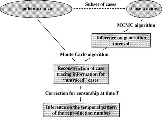
Statistical framework used to estimate the reproduction number with data (epidemic curve and subset of traced cases) available up to time T. To handle uncertainty about the generation interval, a Markov chain Monte Carlo (MCMC) algorithm is set up to investigate the posterior distribution of the generation interval given case tracing data. The output of the MCMC is then used in a Monte Carlo algorithm to make an inference about complete case tracing up to time T. Eventually, a correction is applied for the censorship of late secondary cases during the course of the epidemic.
A decision rule to reinforce control measures.
Assume that control measures are implemented at time TCM (<T). Here, we propose a decision rule to determine whether control measures are efficacious (R < 1), whether they lack efficacy (R > 1), or whether more data are required for decision.
If, in interval Δ⊂[TCM,T], there is high predictive probability that RΔ < 1, efficacy of control measures should be concluded, whereas lack of efficacy should be concluded if there is low predictive probability that RΔ < 1. To make this rule operational, we choose two thresholds s1 percent, s2 percent (s1 < s2) and conclude lack of efficacy when the predictive probability P(RΔ < 1) is <s1 and efficacy when P(RΔ < 1) is >s2. If s1 ≤ P(RΔ < 1) is ≤s2, the conclusion is delayed until more data are available.
We divided interval [TCM,T] into three equal-sized intervals
Simulation of SARS-like outbreaks
A simulation study of SARS-like outbreaks was used to investigate the operating characteristics of the proposed decision rule. Control measures were implemented on day TCM = 20 days. The mean reproduction number before TCM was 3. Four scenarios were simulated, with a mean reproduction number after TCM equal to 0.5, 0.7, 1.1, or 1.3. Case tracing was simulated for 5 percent of the cases. For each scenario, 300 epidemics were simulated. Simulations are detailed in appendix 3.
In a first stage, the estimation method is used to analyze a single epidemic, simulated with R = 0.7 after control measures. The posterior distribution of the generation interval, the predictive mean, and the 95 percent credible interval of the temporal pattern of R are given according to time T of the last observation.
In a second stage, we give, for each scenario, the probability that control measures are said to be efficacious; that control measures are said to lack efficacy; or that more data are required, 2 and 3 weeks after control measures are implemented.
RESULTS
Real-time surveillance of an epidemic
Collected data.
In figure 2, parts (a) and (b) show the simulated data. Part (a) shows the daily rate of case onset. A total of 2,086 subjects were infected, with a peak incidence at day 28.
![Monitoring of a severe acute respiratory syndrome–like outbreak using simulated data. Daily rate of case onset (part a) and cumulative number of traced cases (part b). In the simulation, the reproduction number was 3 before day 20 and 0.7 after; case tracing was available for 5% of the cases. Mean (part c) and standard deviation ((SD), part d) of the generation interval (GI) derived from case tracing data, according to time T of the last observation (solid line: posterior mean; dotted lines: 95% credible interval; dashed line: simulation value). Part (e): expectation (solid line) and 95% credible interval (dotted line) of the reproduction number R calculated for the last 10 days of observation (over the period [T-10, T-3]), according to time T of the last observation; dashed line, simulation value.](https://oup.silverchair-cdn.com/oup/backfile/Content_public/Journal/aje/164/6/10.1093/aje/kwj274/2/m_amjepidkwj274f02_lw.jpeg?Expires=1716508602&Signature=cgguGIO115l9tvuRMVKOwVj-RhncOy-CNyEwraRAnwp-nWwL9xAOTkCNvyNu0bZx7wEsxaiirp4QfPSZY7JL2oLtjk6zNkWYqrPnhRxerAo2zX5NHZszrdUtk1cBFYt55Uh8Xfg3g-WjbU1cbf1hKkDdFTZB2jzy2nqUMDdgdh1RxSsbbTHG1XFMSA6WQ5parPMxYwq5VdRVobRL0ScrQuWlwK-BT1AlmwxrbGFFSex6lyOYPI7Q9SafOPiNP5gwpMRNNvRcQqrU82HJKt4ciPeAhZN3pjfXvTEo6j82vhDxycO10NmRNgzQlDsUKIg-7U1ai8JsxK~bOOKvRZTWNQ__&Key-Pair-Id=APKAIE5G5CRDK6RD3PGA)
Monitoring of a severe acute respiratory syndrome–like outbreak using simulated data. Daily rate of case onset (part a) and cumulative number of traced cases (part b). In the simulation, the reproduction number was 3 before day 20 and 0.7 after; case tracing was available for 5% of the cases. Mean (part c) and standard deviation ((SD), part d) of the generation interval (GI) derived from case tracing data, according to time T of the last observation (solid line: posterior mean; dotted lines: 95% credible interval; dashed line: simulation value). Part (e): expectation (solid line) and 95% credible interval (dotted line) of the reproduction number R calculated for the last 10 days of observation (over the period [T-10, T-3]), according to time T of the last observation; dashed line, simulation value.
Part (b) presents the cumulative number of traced cases. Twelve cases were traced after 3 weeks, 36 after 4 weeks, and 61 after 5 weeks. In total, 114 cases were traced during the epidemic.
Posterior distribution of the generation interval.
Figure 2 also shows the posterior mean and 95 percent credible interval of the mean (part c) and standard deviation (part d) of the generation interval according to time T of the last observation. The Markov chain Monte Carlo algorithm did not converge for T < 14 days because there were ≤3 traced cases.
For both the mean and standard deviation of the generation interval, the 95 percent credible intervals shortened as the number of traced cases increased.
The mean of the generation interval was slightly biased for small values of T. Its posterior mean was 6.5 days (T = 21 days), 7.0 days (T = 28 days), 7.7 days (T = 35 days), and 8.4 days (T > 50 days) for a simulation value equal to 8.4 days.
Temporal pattern of the reproduction number.
In figure 2, part (e) shows the expectation and 95 percent credible interval of the reproduction number calculated for the last 10 days of observation, according to time T of the last observation.
Real-time estimates of R could be computed only once the posterior distribution of the generation interval was available, that is, for T ≥ 14. The real-time expectation of R remained close to its simulation value, irrespective of T.
Evaluating the efficiency of control measures
Table 1 gives the probability that control measures are said to lack efficacy; that control measures are said to be efficacious; or that more data are required, after 2 and 3 weeks, according to the mean reproduction number R.
Posterior probability (%) that control measures are said to lack efficacy, that control measures are said to be efficacious, or that more data are required, after 2 and 3 weeks, according to the mean reproduction number R*
After 2 weeks | After 3 weeks | |||||||||
|---|---|---|---|---|---|---|---|---|---|---|
| Lack of efficacy | More data required | Efficacy | Lack of efficacy | More data required | Efficacy | |||||
| R = 0.5 | 1.8 | 30.6 | 67.6 | 0.3 | 7.3 | 92.4 | ||||
| R = 0.7 | 7.2 | 71.0 | 21.8 | 1.8 | 14.7 | 83.5 | ||||
| R = 1.1 | 77.9 | 20.7 | 1.4 | 71.6 | 23.6 | 4.8 | ||||
| R = 1.3 | 89.7 | 8.9 | 1.4 | 89.7 | 8.5 | 1.8 | ||||
The decision rule is based on the predictive probability p that R < 1: if p < 5%, control measures lack efficacy; if p > 95%, control measures are efficacious. Otherwise, more data are required.
When control measures lack efficacy (R ≥ 1.1), the probability of making the wrong judgment is less than 5 percent after 2 and 3 weeks. When control measures are efficacious (R ≤ 0.7), that probability is less than 2 percent after 3 weeks but may reach 7.2 percent after 2 weeks.
When control measures are efficacious, a correct conclusion is obtained in 67.6 percent (R = 0.5) and 21.8 percent (R = 0.7) of the simulations after 2 weeks and in 92.4 percent (R = 0.5) and 83.5 percent (R = 0.7) of the simulations after 3 weeks.
When control measures lack efficacy, a correct conclusion is obtained in 89.7 percent (R = 1.3) and 77.9 percent (R = 1.1) of the simulations after 2 weeks and in 89.7 percent (R = 1.3) and 71.6 percent (R = 1.1) of the simulations after 3 weeks.
DISCUSSION
In this paper, we have proposed a statistical framework for real-time monitoring of communicable disease outbreaks. In this context, requiring as few data as possible is desirable in order to limit exposure of data collectors and allow efficient use of resources. The method we proposed simply used the epidemic curve and a subset of traced cases. The approach required no prior knowledge of the disease and could therefore be used for emerging communicable diseases.
The existence of a deterministic threshold (R = 1) with a simple interpretation in terms of control of the epidemic led us to propose formal rules for assessing the efficacy of control depending on this threshold. However, it is possible to define alternative rules; for example, one could assess whether R is decreasing by monitoring the posterior probability of the ratio of R in one period to an earlier one. Defining and evaluating other rules requires further research. The method could also be used to estimate the basic reproduction number R0, which is the mean number of cases generated by a typical infectious person when the entire population is susceptible. This information would naturally arise from the value estimated in the early part of the outbreak, before many people recovered or died.
A natural choice would be to implement the decision rule for the whole postintervention period. However, this choice was not found optimal because 1) daily estimates of R are biased for the first days of the interval (the method smoothes the temporal pattern of R; refer to Cauchemez et al. (10)); and 2) daily estimates of R have a large variance for the last days of the interval (10). Our approach of discarding the first and last days of the interval reduced both the bias and variance of the estimates.
There is a compromise to reach between 1) the capture of the temporal pattern of R and 2) the precision of the estimates for each time period. Since precision increases with the number of symptoms onsets over the time period (10), the second objective contradicts the first one. Consequently, at the peak of the epidemic, it might be possible to estimate R during short periods, whereas, during periods of low incidence, it might be optimal to consider longer time periods.
A number of assumptions were made regarding the epidemic and the data collected. First, we assumed that no cases were imported during the course of the epidemic (H1). If this assumption is violated, the estimate of R will be inflated for the days preceding the arrival of such a case, albeit to a small extent. Next, we assumed that all cases were detected (H2), therefore excluding asymptomatic carriage or underreporting. The effect of underreporting on the estimate of R is not clear-cut: downward bias is likely because undetected cases are discounted from the total offspring of earlier cases. However, at the same time, upward bias may follow because the offspring of an undetected case will be allocated to observed cases. We assumed that secondary cases were always reported after their index case (H3) was by considering w(.) null for negative values. This assumption is required for real-time analysis. It could be violated, especially if the incubation period of the disease is long and variable.
The next two assumptions concerned the generation interval, which was supposed to be unknown at the beginning of the epidemic. We assumed that the parameters defining the generation interval would not change throughout the epidemic (H4). This assumption could be relaxed, at the price of increased variability in the estimates, by restricting estimation to the subset of the most recent traced cases and provided that tracing is carried out throughout the epidemic. In the application, we found that, at the very beginning of the epidemic, it might not be possible to provide estimates because too few cases were traced. Using a more informative prior on the generation interval could be considered, until a few dozen cases have been traced. First estimates of the mean of the generation interval were underestimated, which was expected because the first-generation intervals to be detected are the shortest ones. However, for our simulation, the bias remained small and had little effect on the predictive distribution of the reproduction number. Hypothesis H5 was that a random sample of all cases would be traced, which would not be the case if, for example, long generation intervals were unlikely to be sampled. Adopting a parametric form for the generation interval may make the procedure more robust in this respect. Truncation of the generation interval could also be considered explicitly.
Last, we assumed that, in the absence of an observed epidemic curve and tracing information, all chains of transmission were equally likely (H6). This assumption was required to reconstruct complete case tracing data up to the last observation (9). The framework could be extended to integrate more detailed information regarding the social network when available.
An alternative approach for inference would be to sample from the full Bayesian model (refer to appendixes 1 and 2; in particular, compare equations A5 and A6). However, there is little reason to think that it would improve the results because case tracing data are expected to be the main source of information on the generation interval. The approach would be more difficult to implement (11, 12), with little anticipated benefit. The use of two separate steps (inference on the generation interval from the observed case tracing data, followed by reconstruction of the complete case tracing data) appeared to be more pragmatic. If the epidemic curve significantly improved our knowledge of the generation interval, exploration of the full Bayesian model would reduce credible intervals for the reproduction number, but our approach would remain valid.
In the simulation study, we assumed that dates of symptoms onset and case tracing information were available in real time. In practice, we may expect symptoms onset to be available nearly in real time, with a time lag required for case tracing information. The proposed framework makes it possible to retrospectively add case tracing information.
We have presented a statistical framework for real-time surveillance of emerging infectious diseases. It should be of benefit to public health decision makers who have to determine in real-time whether to reinforce control measures.
APPENDIX 1
Bayesian Hierarchical Model
Level 1.
The first term of equation A1 gives the prior distributions of θ = {γ,η}. Here, we specify vague Exponential priors Exp(0.001) for these parameters.
Level 2.
Level 3.
Following Wallinga and Teunis (9), the third term of equation A1 gives the probability of a completely reconstructed case tracing, where each untraced case is allocated to an observed case.
Level 4.
The last terms of equation A1 constitute the predictive distribution of the late number of secondary cases given the early number of secondary cases and θ. In a previous study (10), we showed that, under the assumption that Xt is Poisson distributed with mean ntλ, where λ has a vague Gamma prior (α = 10−5, β = 10−5), the predictive distribution of
APPENDIX 2
Predictive Distribution of the Temporal Pattern of R
We have to predict
This formulation makes the calculation easier because the first term in the integrand is proportional to the product of levels 1 and 2 of the full Bayesian model, and the second term is the product of levels 3 and 4 of the full Bayesian model.
To draw a sample Y1, …, YN from equation A6, we proceed as follows (15):
Step 1: draw a sample θ1, …, θN from
\(P(\mathrm{{\theta}}{\vert}{\{}O_{j},U_{j}{\}}_{j{\in}K_{T}}),\)defined as the product of levels 1 and 2 of the full Bayesian model.Step 2: for i = 1, …, N, for each untraced case j in JT, draw the day
\(U_{j}^{i}\)of symptoms of his or her primary case given θi and the epidemic curve from level 3 of the full Bayesian model.Step 3: for i = 1, …, N, for each t ≤ T, draw
\(X_{t}^{i{+}}(T)\)given θi and\(X_{t}^{i{-}}(T){=}{\sum}_{j{\in}J_{T}{\cup}K_{T}}1(U_{j}^{i}{=}t)\)from level 4 of the full Bayesian model.
In practice, we draw a sample of size N = 5,000.
APPENDIX 3
Simulation of SARS-like Outbreaks
Simulated epidemics were started with 10 index cases. The generation interval had a Weibull distribution with a mean of 8.4 days and a standard deviation of 3.8 days to reflect SARS (18). Control measures were implemented on day TCM = 20 days. For each case detected before TCM days, the number of secondary cases was drawn from a Negative Binomial with a mean of 3 and a shape parameter of 0.18 (9). Four scenarios were considered in which the mean reproduction number after TCM was r = 0.5, 0.7, 1.1, and 1.3. Accordingly, the shape parameter k was calculated as k = −0.0236r2 + 0.131r, which is consistent with Wallinga and Teunis (9). Case tracing was simulated for 5 percent of the cases. For each scenario, 300 epidemics were simulated.
We chose TCM = 20 days so that, in the scenario consistent with the SARS outbreak in Hong Kong in 2003 (R = 0.7 after TCM) (9), the expected number of cases (n = 1,781) was close to the number observed during the epidemic (n = 1,755) (19).
This study was funded by the EU Sixth Framework Programme for research for policy support (contract SP22-CT-2004-511066).
The authors thank Drs. Peter Dodd and Elizabeth Halloran for their useful comments on the manuscript.
Conflict of interest: none declared.
References
Anderson RM, May RM. Infectious diseases of humans: dynamics and control. Oxford, United Kingdom: Oxford University Press,
De Serres G, Gay NJ, Farrington CP. Epidemiology of transmissible diseases after elimination.
Farrington CP, Kanaan MN, Gay NJ. Branching process models for surveillance of infectious diseases controlled by mass vaccination.
Ferguson NM, Fraser C, Donnelly CA, et al. Public health. Public health risk from the avian H5N1 influenza epidemic.
Jansen VA, Stollenwerk N, Jensen HJ, et al. Measles outbreaks in a population with declining vaccine uptake.
Riley S, Fraser C, Donnelly CA, et al. Transmission dynamics of the etiological agent of SARS in Hong Kong: impact of public health interventions.
Ferguson NM, Donnelly CA, Anderson RM. Transmission intensity and impact of control policies on the foot and mouth epidemic in Great Britain.
Haydon DT, Chase-Topping M, Shaw DJ, et al. The construction and analysis of epidemic trees with reference to the 2001 UK foot-and-mouth outbreak.
Wallinga J, Teunis P. Different epidemic curves for severe acute respiratory syndrome reveal similar impacts of control measures.
Cauchemez S, Boëlle PY, Donnelly CA, et al. Real-time estimates in early detection of SARS.
Cauchemez S, Carrat F, Viboud C, et al. A Bayesian MCMC approach to study transmission of influenza: application to household longitudinal data.
Cauchemez S, Temime L, Guillemot D, et al. Investigating heterogeneity in pneumococcal transmission: a Bayesian MCMC approach applied to a follow-up of schools. J Am Stat Assoc (in press).
Berger JO, Liseo B, Wolpert RL. Integrated likelihood methods for eliminating nuisance parameters.
Gelfand AE. Model determination using sampling-based methods. In: Gilks WR, Richardson S, Spiegelhalter DJ, eds. MCMC in practice. London, United Kingdom: Chapman and Hall,
Rubin DB. Bayesianly justifiable and relevant frequency calculations for the applied statistician.
Gilks WR, Richardson S, Spiegelhalter DJ. Markov chain Monte Carlo in practice. London, United Kingdom: Chapman and Hall,
Lipsitch M, Cohen T, Cooper B, et al. Transmission dynamics and control of severe acute respiratory syndrome.

