Subramanian et al. Respond to “Think Conceptually, Act Cautiously”

The importance of socioeconomic position, measured at multiple levels (e.g., individual, household, area) and across the life course, for studying health disparities is now well recognized (1–7). Our multilevel study (8) reported that individual-based socioeconomic measures (IBSMs) and area-based socioeconomic measures (ABSMs) together capture birth weight inequalities that otherwise would have been missed by considering one or the other. We found additionally that, in the absence of IBSMs, the bulk of birth weight disparities captured by ABSMs was approximately similar to that which would have been captured by IBSMs (8). Geronimus (9) critiques these findings, in part, by (mis)interpreting our study as an examination of how well ABSMs serve as “proxies” for IBSMs, even though we explicitly conceptualized ABSMs as capturing some important mix of individual- and area-level influences on health, thereby providing valuable information on socioeconomic disparities in health (8). In this rejoinder, we elaborate on the fundamental distinctions between our respective approaches to analyzing socioeconomic disparities in health.

MODEL CONCEPTUALIZATION: SINGLE-LEVEL OR MULTILEVEL?

FIGURE 1.

Open in new tabDownload slide

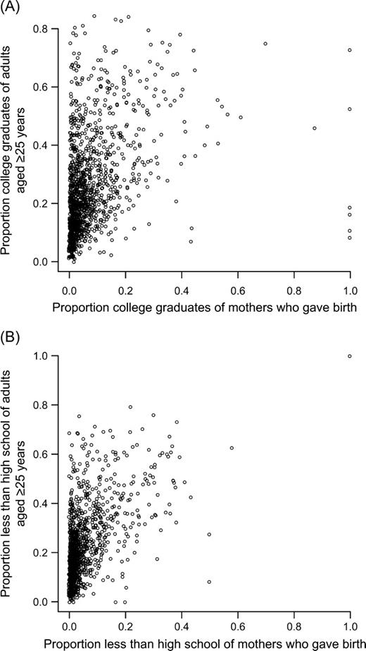
Scatterplots of census tracts showing the proportion of college graduates of all adults aged ≥25 years and the proportion of college graduates of mothers who gave birth (A) and the proportion of the population with less than a high school education of all adults aged ≥25 years and the proportion of mothers with less than a high school education who gave birth of all mothers who gave birth (B), Massachusetts, 1990.

ABSMs: CONTINUOUS OR CATEGORICAL?

Geronimus argues that modeling the ABSM as a continuous predictor (0–100 percent), with linear assumptions, would result in a substantially larger ABSM effect compared with IBSM effect. Consequently, Geronimus claims that our finding that, in the absence of IBSMs, ABSMs approximated or provided a “conservative” estimate of birth weight inequalities is incorrect. The reason that this will occur is simply due to comparing birth weights in areas where 0 percent of the population, for instance, has less than a high school education with areas where 100 percent of the population has less than a high school education. In Massachussetts, in 1990, of the 5,531 census tracts with nonmissing information on poverty (comprising 99.8 percent of the state's total of 5,543 census tracts), only 1 percent (n = 13) had a poverty level of 0 percent, and only 0.1 percent (n = 1) had a poverty level of 100 percent; similarly, only 14 census tracts had a percentage of less than high school education equal to zero, and only one had 100 percent, making the interpretation of a 0–100 percent contrast highly abstract, if not meaningless. Geronimus is correct in observing that there is no inherent correspondence between the individual categories “college graduates” and “less than high school education” with the ABSM categories “<15 percent” and “40 percent or more” with less than a high school education, with respect to comparability of the socioeconomic gradient. However, there is even less inherent correspondence of the individual education categories with the 0 percent and 100 percent contrast that Geronimus recommends. Indeed, a more systematic approach would be to compare extreme categories of IBSMs and ABSMs such that they encapsulate a constant proportion of the population. This approach is similar to the relative index of inequality that was originally developed to compare social class gradients over time, given the changing population proportions captured in the most extreme categories of hierarchy (18). We find that approximately 75 percent of the population was located between the extreme categories used for both our individual-level maternal education measure and the census tract-level “percentage of adults aged 25 years or more with less than a high school education” (using midpoint interpolation to approximate the cumulative distribution function), thereby suggesting that our choice of categories for comparison is more appropriate than the extreme 0–100 percent comparison. Furthermore, comparisons of IBSM and ABSM effects have to recognize the “shape” of their association with health outcome, which if nonlinear (1, 2, 6, 12, 15), as partially substantiated by our results, makes the use of continuous measures (modeled as linear effects) particularly problematic.

ABSMs: SAME OR DIFFERENT?

Geronimus accuses us of overinterpreting the differences in the effect estimates observed for the college education ABSM and those observed for poverty and less than high school education ABSMs, arguing that these are essentially interchangeable. As mentioned in our study (8), there are a priori grounds to anticipate that the college education ABSM (a marker for affluence) need not simply be the opposite of the less than high school education or poverty ABSM (a marker for disadvantage), especially in terms of the mechanisms and processes that the two may generate to influence health (19, 20). As figure 2 shows, areas with low poverty can have very different ranges of the proportion of the population with a college education and vice versa; thus, specificity of socioeconomic measures (IBSM or ABSM) matters. Geronimus incorrectly states that we avoid reporting the socioeconomic differentials in the low birth weight by college education ABSM (refer to figure 1 of the original study (8)).

FIGURE 2.

Open in new tabDownload slide

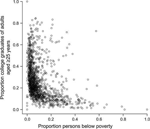
Scatterplot of census tracts showing the proportion of college graduates of all adults aged ≥25 years and the proportion below poverty, Massachusetts, 1990.

SOCIAL DISPARITIES IN HEALTH: ETIOLOGIC OR SURVEILLANCE RESEARCH?

Geronimus (9) disregards research on quantifying and monitoring socioeconomic disparities in health that has no etiologic component. Indeed, by documenting multilevel influences (individual and area) on birth weight, we highlight the somewhat artificial distinction between monitoring/surveillance research and etiologic research. Answering monitoring questions on who, in what type of places, are at the greatest disadvantage for health, besides being important in itself, posits important etiologic questions, such as if ABSM effects are substantial, then what does it tell us about the processes that generate individual- and area-based disparities in health, or are ABSM and IBSM effects synergistic/interactive or are they independent of one another? We concur with the recommendation of Geronimus to encourage efforts to improve data collection and monitoring at the individual level. However, we do not find this effort to be incompatible with use of ABSMs that is facilitated through geocoding of the health events obtained from public health data. From a practical perspective, it is important to note that the lack of IBSMs (not to mention the quality of these measures, including missingness) in many public health surveillance databases is likely to continue. Within this context, we view the use of ABSMs as complementing, not supplanting, any efforts to improve collection of IBSMs in public health surveillance data (4, 15, 21–23).

Notwithstanding the dismissive tone of Geronimus' critique (9), the field of population health is adequately poised for a constructive discussion on the science of studying ABSMs (4, 10, 12, 24).

S. V. Subramanian is supported by National Heart, Lung, and Blood Institute Career Development Award 1 K25 HL081275 from the National Institutes of Health.

Conflict of interest: none declared.

References