


Abstract
Mild mental impairment (MMI) represents the low extreme of the quantitative trait of general intelligence and is highly heritable. Quantitative trait loci (QTLs) conferring susceptibility to MMI, as for most complex traits, are likely to be of small effect size. Using a novel approach we call SNP-MaP (SNP Microarrays and Pooling), we have identified four loci associated with MMI. These four loci have been replicated in two SNP-MaP studies and verified by individual genotyping. The two SNP-MaP studies conducted were a case versus control comparison (n=515 and n=1028, respectively) and a low versus high general intelligence extremes group comparison (n=503 and n=505, respectively). Each of the four groups consisted of five independent ‘subpools’, with each subpool assayed on a separate microarray. Twelve loci showing the largest significant differences in both SNP-MaP studies were individually genotyped on 6154 children. Of the four loci positively associated with MMI, the minor allele of each conferred the greater risk for MMI. Two of the loci are close to known genes and may be in linkage disequilibrium with them. One of the loci is between the candidate genes KLF7 and CREB1, but given possible long-range effects on expression and the unknown importance of untranslated elements such as micro-RNAs, all four loci deserve attention as candidates. Although each SNP accounts for a small amount of variance, their effects are additive and they can be combined in a ‘SNP set’ that can be used as a genetic risk index for MMI in behavioral genomic analyses.
GenBank accession nos BC038530 and AF217510
INTRODUCTION
Mental retardation is a spectrum of learning impaired disorders marked by low IQ and problems with adaptive behavior. It is categorized by DSM-IV (1) into three distinct groups of increasing impairment and rarity: profound (IQ<20–25), severe (IQ 20–25 to 35–40) and moderate (IQ 35–40 to 50–55), with the incidence of IQs lower than 50 less than 0.5% (2). A recent analysis of the Online Mendelian Inheritance in Man (OMIM; http://www.ncbi.nlm.nih.gov/entrez/query.fcgi?db=OMIM) database indicates that 280 unrelated chromosomal aberrations and single-gene mutations involve or cause mental retardation (3) but are uncommon in the general population (4). Although severe mental retardation has drastic consequences for the affected individual, mild mental impairment (MMI), defined as IQs from 55–60 to 70–75, has a larger cumulative effect on society because many more individuals are affected. Even though most MMI individuals can live independently and hold a job, the prevalence of MMI is an issue of increasing concern as society continues to become more technologically dependent (5).
Two large family studies suggest that MMI is familial (6,7). The first twin study, from which the present report emanates, showed that MMI has a group heritability of ∼50%, indicating that half of the phenotypic variation of intelligence is explained by genetic variation (8). This twin study also indicated genetic links between MMI and variation in the normal range of intelligence—a finding compatible with the quantitative trait loci (QTL) hypothesis that MMI is caused by the same multiple genes that operate throughout the distribution of general intelligence (‘g’) (8,9). The molecular genetics of MMI is still in its infancy and so far only one QTL has been nominated (10), a SNP (rs1136141) in the 5′-untranslated region of a heat shock protein gene (HSPA8). This QTL association accounts for less than 0.5% of the variance, which demonstrates that the 1% QTL effect size barrier (11) can be broken. It is possible that many QTLs for complex traits such as ‘g’ are of similarly small effect size.
The ability to detect QTLs of small effect size requires large samples. For example, 80% power (P<0.01, two-tailed) to detect an effect of 0.5% in an unselected sample requires samples of at least 1000 individuals (12). The need to genotype large samples tends to result in research on a small number of candidate genes as has happened in research on ‘g’ (13). However, systematic association studies, especially whole-genome association studies, require very large numbers of DNA markers, most likely, hundreds of thousands of SNPs (14,15). The problem is that genotyping large samples for large numbers of SNPs is extremely costly.
One solution to reduce the cost, time and labor involved in genotyping large samples is to perform analyses not on individual DNA samples but on pools made up of DNA from groups of individuals such as case versus control groups (16). The advantage of DNA pooling is that it can screen for QTL associations quickly and efficiently; by pooling individuals' DNAs, genotyping efforts are reduced by a function of the number of individuals in the pools. DNA pooling has previously been validated using both microsatellites (17–20) and SNPs (21–27). Because individual genotypes cannot be determined from genotyping pooled DNA, analyses compare allele frequency differences between groups using fluorescent hybridization/peak-height signals. For this reason, allele frequency measurement in DNA pools is ‘allelotyping’ rather than ‘genotyping’.
One disadvantage of DNA pooling—as with individual genotyping—is that set-up costs per SNP are quite high because each marker requires PCR reagents and specific oligonucleotide primers. An exciting development to reduce such costs in genotyping large numbers of SNPs is the recent introduction of microarrays. Microarrays permit SNP genotyping by using thousands of oligonucleotides on a small scannable surface. The present research employs the Affymetrix GeneChip® Mapping 10 K Array Xba 131 microarray that uses a one-primer assay to genotype over 10 000 SNPs on a single microarray. The average call rate for the 10 K GeneChip is >95%, reproducibility (when compared with other GeneChip assays) is >99.9% and accuracy (when compared with single assay genotyping) is >99.5% (28). The median inter-SNP distance on the Affymetrix 10 K GeneChip is 105 kb.
Although microarrays can be used to genotype large numbers of SNPs, they are expensive to use to genotype large numbers of individuals because each microarray can be used only once. We have combined the strength of DNA pooling to genotype large numbers of individuals and the strength of microarrays to genotype large numbers of SNPs by allelotyping pooled DNA on SNP microarrays, a technique that we call ‘SNP-MaP’ (SNP Microarrays and Pooling). Although SNP microarray technology was designed for qualitative genotype-calling of individuals, we have successfully allelotyped pooled DNA for 100 individuals on the Affymetrix GeneChip Mapping Array (29). To our knowledge, only one previous report has attempted to genotype pooled DNA on microarrays in the search for QTLs (30). Allele frequency estimates were obtained using a microarray designed to interrogate 7283 SNPs in 71 candidate gene regions over 17.1 Mb in order to identify associations using pooled groups based on low and high HDL cholesterol levels. In contrast, the current study is the first application of the SNP-MaP technique for genome-wide screening. The current study also differs in that we employ multiple subpools for each group to estimate sampling variance as well as a replication SNP-MaP design to nominate SNPs for individual genotyping. Although at least 100 000 SNPs are needed for even a coarse genome scan for association (14,15), our use of 10 000 SNPs means that at best we could detect one-tenth of QTL associations. The distribution of QTL effect sizes is not known for any complex trait, but if the 50% heritability of MMI were caused by QTLs with average effect sizes of 0.5%, this would suggest 100 QTLs and we might be able to detect 10 of them with the 10 K microarray.
Design
Our sampling frame included more than 6000 children in 3000 twin pairs with cognitive data obtained at 7 years of age and with DNA previously collected as part of the Twins Early Development Study (TEDS) (31). In order to maximize statistical power efficiently, we selected the extremes and controls; to reduce false positive results, we conducted two studies using pooled DNA. The first study (‘study 1’) used a case versus control design with 515 MMI cases and 1028 representative controls. The second study (‘study 2’) used a low versus high design with 503 individuals who were in the low extreme of general intelligence (but not MMI cases) and 505 individuals from the high extreme of the ‘g’ distribution. Only one member of a twin pair was selected for a group so that all individuals in a study were genetically independent. For each of the four groups, individuals were randomly divided into five ‘subpools’ in order to estimate sampling variance for each group. Each subpool was assayed on a separate microarray. We used a correction factor (32) to protect estimates of allele frequency from DNA pools against unequal allelic signal detection based on previous work (33). SNPs nominated on the basis of the two SNP-MaP studies using pooled DNA were individually genotyped for a sample of 6154 TEDS children. Data from individual genotyping were used to test the SNP-MaP results and to test for QTL associations across the entire sample.
RESULTS
Reliability of pooled DNA estimates from microarrays
Of 11 560 SNPs on the microarray, SNP-MaP estimates were derived for the following number of SNPs for each group: 11 318 (cases), 10 729 (controls), 11 022 (lows) and 10 181 (highs) generated from at least four of the five microarrays per group. To index allele frequency in DNA pools, the two quantitative relative allele signal (RAS) scores (RAS1 and RAS2)—generated from the microarray analysis software—were corrected (RAS1′ and RAS2′) and averaged (RAS′av). RAS′av values were highly correlated across the five DNA subpools; for the case group, pairwise correlations across the five microarrays were between 0.945 and 0.962; 0.913 and 0.948 for the control group; 0.931 and 0.952 for the low extreme group and 0.839 and 0.935 for the high extreme group. Similarly, mean allelic frequency differences between subpools were generally small: 0.056–0.066 (cases), 0.064–0.083 (controls), 0.062–0.075 (lows) and 0.071–0.113 (highs).
From the two SNP-MaP studies, 12 SNPs were selected for individual genotyping (discussed subsequently). Individuals for whom individual genotyping data were available were reconstituted into the four groups to confirm the accuracy of the allele frequency estimates from microarrays. A correction coefficient, k (see Materials and Methods), was unavailable for two SNPs (rs2254209 and rs733656) and therefore produced less than optimal absolute allele frequency estimates. After removing these two SNPs, mean differences between SNP-MaP estimates and individual genotyping were 0.033 (cases), 0.045 (controls), 0.052 (lows) and 0.057 (highs). The discrepancies between estimates for pooled DNA and individual genotyping diluted the difference between groups in analyses of the individual genotyping data. Nonetheless, the average correlation for all groups between microarray estimates of pooled DNA and individually genotyped estimates was 0.973, confirming our previous results suggesting that the SNP-MaP approach to allelotyping is highly reliable (29).
SNP-MaP results for study 1 and study 2
SNP allelotype comparisons could be made for 10 681 SNPs in study 1 and for 10 092 SNPs in study 2. Figure 1A and B shows scatter plots comparing k-corrected allele frequencies for the two groups in both studies. The correlations between cases and controls and between lows and highs were 0.984 and 0.970, respectively. These high correlations demonstrate that the reliability of estimating allele frequencies with pooled DNA. Reflecting the high correlations between groups, mean group differences in allele frequency estimates were relatively small (0.038 for study 1 and 0.48 for study 2). Outliers indicate differences between cases and controls (Fig. 1A) and between low and high extremes (Fig. 1B).
A t-test for independent samples with five subpools was used to test the significance of group differences (case versus control and low versus high groups) for each SNP. We used a nominal P-value of 0.03 that involved an allelic frequency difference of about 0.07 between groups, depending on the sampling variance of each SNP. Because power is substantially reduced for low frequency alleles, SNPs were removed if they showed a minor allele frequency less than 0.10 in one or both groups in each study. SNPs were of course required to show group differences in the same direction across the two studies. The number of SNPs meeting these criteria was 222 in study 1 and 227 in study 2. SNP-MaP differences in study 1 and study 2 for the 222 significant SNPs in study 1 correlated 0.807. Similarly, a correlation of 0.806 was observed when correlating SNP-MaP differences in study 1 and study 2 for the 227 SNPs significant in study 2. Although these results indicate substantial correspondence between the results of study 1 and study 2, only 12 SNPs met our severe criterion requiring significance in both studies. These SNP-MaP results are shown in Table 1. The average difference between groups is small, 0.073 for study 1 differences and 0.079 for study 2 differences, but more than twice as large as the standard errors of the mean, as expected by the significance of their differences.
By comparison, after removing SNPs whose results were not in the same direction across the two studies and SNPs with minor allele frequencies <0.1, using combined P-values across the two studies suggests that 75 SNPs should be followed up for individual genotyping (P∼0.007; see Materials and Methods). It should be noted, however, that only the 12 SNPs we selected were significant in both studies; in many cases, the other 63 SNPs were very highly significant in one study but not nearly significant in the other study. Interestingly, if we apply a step-down false discovery rate (FDR) (34) of 5% to the study 1 P-values, we expect only one SNP to be a true discovery, i.e. the most significant SNP (P=1.2×10⁻⁶). As we are looking for QTLs of small effect, this improbable outcome is a reflection of modest between-group differences that results in their correspondingly moderate (rather than extremely low) P-values across SNPs. Moreover, if only one SNP survives the FDR procedure, the threshold for its significance is algebraically equivalent to the overly conservative Bonferroni correction procedure. Importantly, this SNP in study 2 was non-significant (P=0.102), suggesting it may be a false positive result. For this reason, we prefer to rely on our replication SNP-MaP design as a more conservative criterion for selecting SNPs for individual genotyping.
The aim of the SNP-MaP method is to genotype a large number of SNPs using pooled DNA in order to nominate SNPs for individual genotyping, which provides the confirmation of QTL association using standard statistical tests. For each of the 12 candidate SNPs nominated by SNP-MaP (Table 1), we individually genotyped more than 6000 children to test whether the QTLs nominated at the extremes of the distribution in our SNP-MaP studies also meet the QTL criterion of showing an association throughout the entire range of variation.
The 46 076 genotypes from 2057 MZ twins and 3183 DZ twins for 11 SNPs (excluding rs2254209 which showed high individual genotyping error) were entered into a Pedigree file and analyzed using Merlin and QTDT software. QTDT (35) implements the variance-components model (36,37) that takes into account the family structure (in our case, twin pair structure) of the data, yielding estimates of association within pairs that control for population stratification and association between pairs that is comparable to associations for all individuals but taking into account the correlations within twin pairs. The ‘Total Association’ model, which provides an overall test of association, revealed four SNPs (rs991684, rs4128492, rs2382591 and rs726523) significantly associated with ‘g’ (Table 2). Repeating this analysis using the less powerful ‘Within’ model, which only considers the within-family component of association by comparing Mu (null model) to Mu+within-twin variances (full model), reveals just one significantly associated SNP (rs726523; χ2=4.69, P=0.030). The lack of concordance between significant SNPs in the Total Association and Within models is probably due to reduced power caused by a reduced number of probands in the Within model (which is restricted to using only informative DZ pairs) rather than population stratification effects. This interpretation is bolstered by running the QTDT ‘Population Stratification’ model. In this model, which tests for stratification effects by comparing the between and within components of association, no significant effects of population stratification were found for any SNP.
Table 3 and Figure 2A–D show the effects of the three genotypic groups on standardized ‘g’ scores for the four SNPs significant in the QTDT ‘Total Association’ analysis. The results show a clear additive relationship between genotype and phenotype for all but one SNP (rs2382591); the large error bars for the AA genotype for this SNP reflect the small sample size of this genotypic group, the smallest group by far (n=156). Ignoring this effect for SNP rs2382591, we used an additive genetic model (AA=0, AB=1, BB=2; alleles coded alphabetically) to correlate genotype with standardized ‘g’. As shown in Table 3, all genotype-by-phenotype correlations were significant, although their effect sizes were very small. The largest correlation (for rs991684) is only 0.06, which accounts for 0.36% of the variance. Similarly, the standardized ‘g’ score difference between the homozygotes AA and GG for rs991684 is 0.16; because these are standardized scores, this indicates that the difference is 0.16 of a standard deviation. The significant association for rs2382591 with ‘g’, despite the apparent heterozygote effect depicted in Figure 2C, is a reflection of large samples for the two most common genotypes. The negative correlation for SNP rs41284924 indicates lower scores for the G allele of the A/G SNP. Effect sizes (r2) shown in Table 3 reflect the results of the QTDT analyses. As expected from the genotypic values shown in Figure 2, use of non-additive genotypic values (dominance) did not improve the results.
Additive genotypic values for the SNPs were uncorrelated (i.e. not in linkage disequilibrium), as expected because the SNPs reside on different chromosomes (Table 2). This permitted the creation of a ‘SNP set’ that aggregates the small effects of each SNP. Genotypes were coded 0, 1 or 2 with 0 conferring lowest ‘g’ (MMI) and 2 conferring highest ‘g’. SNP genotypes for the four significant associations were summed to produce SNP-set scores, 0 through eight, for 4866 twins for whom complete data were available. SNP-set scores were normally distributed with only modest skew (−0.412), reflecting the finding that the minor allele in each case confers lower ‘g’ (Fig. 3).
As indicated in Figure 3, no children had SNP-set scores of 0 and only three children had SNP-set scores of 1. The correlation between SNP-set scores and ‘g’ is 0.087 and highly significant (P=6×10⁻¹⁰, one-tailed), indicating an effect size (0.076%) that is nearly the sum of the effect sizes of the four SNPs shown in the last column of Table 3. Figure 4 shows the relationship between SNP-set scores 2–8 and standardized ‘g’ scores. The SNP-set scores show a linear relationship with ‘g’ scores, especially for SNP-set scores 4–8 where the sample sizes are larger, as indicated by the ±1 SEM error bars. The average ‘g’ score for children with SNP-set scores of 2 is −0.42 and the average ‘g’ score for children with SNP-set scores of 8 is 0.18. Thus, the average ‘g’ difference between the lowest and highest SNP-set scores is 0.6 of a standard deviation, an effect size comparable to nine IQ points. Use of non-additive genetic models (epistasis) did not improve the results.
DISCUSSION
In this first application of the SNP-MaP approach, we allelotyped pooled DNA for groups selected from 6154 children using single-primer, rapid-protocol 10 K SNP microarrays in two studies of MMI to screen for SNPs showing significant between-group allele frequency differences. Association was then tested by individually genotyping these nominated SNPs in a sample of 6154 MZ and DZ twins in order to detect QTLs of small effect size that operate throughout the distribution. Using this SNP-MaP strategy to nominate SNPs followed by individual genotyping to confirm QTL associations, we have identified four SNPs significantly associated with MMI. These QTL associations appear to be the smallest significant QTL effect sizes detected to date, from 0.10 to 0.36%, suggesting that QTL effect sizes may be much smaller than generally recognized which means that even larger samples are needed to detect them. Nonetheless, we showed that these small QTL effects can be aggregated in a ‘SNP set,’ which sums the effects of the QTLs (accounting for 0.076% of the total variance in ‘g’ scores) and yields a linear relationship with ‘g’ scores across the distribution.
In the following sections, we begin by discussing the SNP-MaP approach and then provide more detail about the four SNPs that we found to be associated with MMI. We also discuss the utility of SNP sets and implications of our findings in relation to QTL effect sizes.
SNP-MaP
The value of the SNP-MaP approach is its efficiency in screening large numbers of SNPs for large numbers of individuals. Our SNP-MaP design that includes four groups in two studies with five subsamples for each group used 20 microarrays with a total cost of ∼$20 000. Individually, genotyping 12 SNPs for 6154 individuals cost $10 000. This total cost of $30 000 can be compared to the cost of ∼$10 million for genotyping the 6154 individuals using a one-assay-per-SNP approach or ∼$5 million for genotyping each individual on the 10 K microarray. By screening 10 000 SNPs in just 20 microarray assays using pooled DNA, we were able to nominate 12 SNPs to be tested using individual genotyping and cut costs several hundredfold.
Four SNPs associated with MMI and ‘g’
Four of the 12 SNPs selected for individual genotyping showed associations with MMI in study 1 and study 2 and with ‘g’ in a QTL analysis of the entire unselected sample. Finding SNP associations across these three studies increases confidence in these findings, although further replication is important. However, although one SNP (rs991684) maps to a region characteristic of a gene (discussed subsequently), the other three SNPs are not located in genes, which might decrease confidence in these findings. As explained later though, two of the three SNPs are near interesting genes.
It is interesting that for each SNP, the rare allele is associated with MMI. One possibility is that there is a selective disadvantage for alleles associated with MMI. Three of the SNPs (rs991684, rs4128492 and rs2382591) show significant deviation from Hardy–Weinberg equilibrium suggesting that selection is a factor. However, the genotypic frequency differences are very small, and significance may be due to the large sample size employed.
rs991684 (located on 2q33.3) shows the largest independent effect size of the four significant SNPs. There is both EST and mRNA evidence that rs991684 maps to the third intron at the 5′ end of a gene of unknown function. The gene spans 16.97 kb, contains five exons, and is expressed at a low level in the medulla. The sequence of this gene has been supported by two sequences from one cDNA clone (GenBank accession no. BC038530) and produces one transcript with one complete product, 1026 bp in length. We are currently exploring this region further.
When analyzing haplotype blocks from the HapMap Caucasian dataset defined using confidence intervals of linkage disequilibrium (38) [implemented in Haploview (39)], rs991684 is found to be in a haplotype block of 26 kb containing nine SNPs. rs991684 is in close proximity (∼200 bp upstream) to a conserved transcription factor binding site, known to bind Cartilage homeoprotein 1 (CART-1) which suggests an obvious next step for further investigation. Indeed, we find 27 conserved transcription factor binding sites captured within the 26 kb haplotype block. In general, the vast majority of a 5 Mb window around rs991684 shows sequence conservation across chimp, mouse, rat and dog, and, as expected, synteny of the two genes flanking rs991684 (KLF7 and CREB1) is observed across all four species. Such long sequences of conservation have previously been linked to functional elements (40,41), which suggest this SNP may be in a functional region if it is not itself a gene.
Another possibility is that rs991684 is in linkage disequilibrium with a QTL. rs991684 is upstream of the start sites of two known genes: 68.8 kb from Kruppel-like factor-7 (KLF7) and 295 kb from cAMP responsive element binding protein 1 (CREB1). Given the distance from KLF7, it is not surprising that rs991684 is in linkage disequilibrium with several KLF7 variants. KLF7 is expressed in both brain and peripheral nervous system and is one of 15 KLF family members of the zinc finger proteins; it has been implicated in vertebrate development as well as controlling cell proliferation, growth and differentiation (42). CREB1 is also expressed in the brain and peripheral nervous system and has been shown to play an important role in memory formation by encoding a regulatory unit necessary for long-term facilitation (43). However, there is no evidence of linkage disequilibrium between rs991684 and CREB1.
The SNP showing the second largest effect size was rs726523 (18q22.1). Using the confidence interval interpretation of HapMap (38), it lies in a haplotype block of 28 kb with nine other SNPs, eight of which show complete linkage disequilibrium with rs726523. Linkage disequilibrium with rs726523 does not extend beyond the 28 kb haplotype block. Moreover, in the 500 kb sequence surrounding rs726523, there are 38 haplotype blocks, with a mean block size of 9 kb, possibly indicating multiple recombination hotspots in this region. Using Multiz alignments (44) to measure conservation, the bulk of a 500 bp region centered on rs726523 can be aligned with chimp and dog, but not mouse, indicating possible functional significance. The nearest conserved transcription factor binding site is ∼97 kb away, outside of its 28 kb haplotype block (discussed previously). The nearest gene, chromosome 18 open reading frame 4 (C18orf4), lies 412 kb downstream and shows no evidence of linkage disequilibrium with rs726523. Although rs726523 is not in linkage disequilibrium with any known protein-coding gene, this does not necessarily mean that its significant association with MMI is spurious. For instance, it is possible that intergenic DNA plays a regulatory role (45).
SNP rs4128492 is located on chromosome 6q25.3 in close proximity to three protein coding genes: 116 kb upstream from AT-rich interactive domain 1B (ARID1B), 24.9 kb upstream from chromosome 6 open reading frame 35 (C6orf35) and 24 kb downstream from zinc finger DHHC domain-containing 14 (ZDHHC14). rs4128492 shows significant and substantial linkage disequilibrium (D′=0.85) with one marker (rs2800451) in the 5′-intronic region of ZDHHC14, a gene involved in metal ion binding, and warrants further investigation. In addition to this, rs4128492 shows modest and non-significant linkage disequilibrium (D′>0.6) with 12 other polymorphisms in ZDHHC14. C6orf35 is an open reading frame with a known protein product (GenBank accession no. AF217510) of unknown function. Unfortunately, neither of the two SNPs in C6orf35 genotyped by HapMap, have been genotyped in the CEPH population, which would have permitted linkage disequilibrium analysis with rs4128492. ARID1B is associated with protein binding and transcription co-activator activity by chromatin-regulated transcription maintenance (46). Constructing haplotype blocks using the ‘four-gamete’ rule (47) allocates rs4128492 to a haplotype block containing two 3′-intronic markers (rs7751698 and rs7740724) in the ARID1B gene, although linkage disequilibrium is not strong between rs4128492 and these two markers. In the immediate vicinity of rs4128492, there is high sequence conservation with chimp and dog but none with mouse or rat. Interestingly, ARID1B and C6orf35 flank a conservation desert spanning ∼50 kb, which is of unknown functional consequence. The conservation of ARID1B, C6orf35 and ZDHHC14 typify this genomic region; ∼10% of the 5 kb surrounding rs4128492 is conserved in chimp, mouse, rat and dog with the largest conserved sequence <300 bp. It has been postulated that small-length (<1 kb) sequences conserved in multiple species may indicate functionality (48), although this hypothesis has been explored primarily in relation to exonic regions. In addition, the haplotype block that contains this SNP (discussed previously) includes 27 conserved transcription factor binding sites, the closest being ∼1.7 kb from the SNP. Thus, investigating transcription factor binding sites may be another profitable direction to elucidate the role of this SNP.
Finally, SNP rs2382591 resides on chromosome 7q11.21 close to the centromere. Confidence interval rules of linkage disequilibrium put rs2382591 in a large (226 kb) haplotype block with strong linkage disequilibrium stretching over the entire block, as often occurs near the centromere. There are no genes within 1 Mb of rs2382591 and the region is not evolutionarily conserved. As with rs726523, it is possible that such intergenic SNPs have as yet unknown regulatory effects. Regardless of understanding the mechanisms by which these SNPs have their effect on ‘g’, if these SNP associations with ‘g’ are real, they can be used as a genetic risk index, as discussed in the following section.
SNP set
SNP sets, or QTL sets more generally, can be useful in three ways. First, just as we aggregate items on a scale to produce a more reliable measure, aggregating QTLs will also produce a composite that is more reliable for predicting complex traits than the individual QTLs. This principle of aggregation is likely to improve the replicability of QTL results. Secondly, QTL sets are cumulative in the sense that new QTLs can be added to a QTL set that increasingly accounts for the heritability of a trait. For example, we are currently using the Affymetrix 100 K GeneChip, which became commercially available in June 2004, with the expectation that a 10-fold increase in the number of SNPs will result in a 10-fold improvement in our ‘g’ SNP set. That is, because 100 K evenly distributed SNPs will show little linkage disequilibrium (although the 500 K microarray under development at Affymetrix is likely to reach a ceiling of linkage equilibrium), we expect to identify a SNP set with 40 SNPs that accounts for as much as 8% of the variance, which is about 1/6 of the total genetic variance of ‘g’. Moreover, QTLs can be added to a QTL set from any source not just from SNP-MaP. For example, QTLs identified from candidate gene analyses of gene networks (49) could be added to a QTL set such as our ‘g’ SNP set. Finally, QTL sets will be useful as genetic risk indices in top-down research on complex traits such as behavior that focus on the whole organism to investigate such questions as diagnosis (e.g. heterogeneity and comorbidity), development (the earliest age at which associations can be found) and the interface between genes and environment (GE correlation and interaction). We are using our SNP set for ‘g’ at 7 years in behavioral genomic analyses that capitalize on the longitudinal and multivariate dataset of TEDS (50). This top-down approach in behavioral research has been called behavioral genomics (51) to distinguish it from bottom-up approaches with which the term functional genomics is usually associated. QTL sets are less useful for bottom-up approaches because the molecular biology of each QTL will be different, although incorporating the QTLs from a QTL set in a multivariate perspective is likely to illuminate coordinated pathways between QTLs and behavior because these QTLs have a common phenotypic effect. Similarly, a multivariate approach to behavioral genomic analyses that examines individual QTLs within a QTL set could identify different profiles of associations — in effect, different QTL sets — for different purposes. For example, different weightings of the SNPs in our ‘g’ SNP set at 7 years of age might predict the earliest developmental emergence of associations or correlations and interactions between the SNP set and measures of the environment.
An important practical implication of the use of QTL sets as genetic risk indicators in behavioral genomic research is that they can be used in samples of reasonable size, which is important, for instance, in research such as neuroimaging for which large sample sizes are not feasible. For example, the average effect size of the four SNPs in our current ‘g’ SNP set is only 0.2% which requires a sample size greater than 2500 for replication with 80% power (P<0.01, one-tailed) (52). In contrast, our SNP set, which accounts for 0.76% of the variance, would require a sample of about 700 for replication with 80% power (P<0.01, one-tailed) (52). Moreover, even with this weak effect size, much smaller samples can be studied if a QTL set can be used for genotypic selection, although genotypic selection requires the availability of a large sample genotyped for the QTLs in the QTL set. As noted in relation to Figure 4, the average ‘g’ difference between the lowest SNP-set scores of 2 and the highest SNP-set scores of 8 is greater than half a standard deviation. Genotypically selected samples of about 80 in the low and high SNP-set groups will provide 80% power (P<0.01, one-tailed) to detect effects of this magnitude. Moreover, if the 100 K microarray is successful in producing a SNP set of 40 SNPs that accounts for 8% of the variance, the SNP set could be replicated with 80% power in unselected samples as small as 80 individuals; genotypically selected samples (which would be expected to show mean differences of 1.5 standard deviations) could be as small as 10 each in the low and high SNP-set groups. These estimates of sample size pertain to replicating the QTL-set results; greater sample sizes are needed for behavioral genomic analyses, where power is attenuated as a function of the correlation between the target variable for the SNP set (‘g’ in our case) and the other variables in behavioral genomic analyses (e.g. measures of related traits such as reading).
QTL effect size
The complete distribution of QTL effect sizes is not known for any complex trait in any field and may not be knowable if, as seems likely, some QTL effect sizes are so small as to be practically undetectable. Although the 10 K microarray only samples a small proportion of the genome, our SNP-MaP approach using a large sample has identified four SNPs associated with MMI whose average effect size is only 0.2%. If our ongoing work using the 100 K microarray and future work using the 500 K microarray yield similar results, it would suggest that QTL effect sizes for complex traits such as MMI might be much smaller than that previously considered. Although a larger net with more SNPs is likely to catch some QTLs of larger effect size, it also seems likely that there are many QTLs of such small effect size that they will be impossible to detect. For now, it seems reasonable to propose that the target QTL effect size for power calculations should be 0.2%. As mentioned earlier, a 0.2% effect size implies that an unselected sample size greater than 2500 is needed to reach 80% power even with a nominal P-value of 0.01 which by itself provides no protection against the 1000 false positive results to be expected with, for example, a 100 K microarray. Rather than attempting to study a single sample with hundreds of thousands of individuals needed to provide genome-wide protection against false positive results, our tactic is to screen out false positive results using replication designs.
Regardless of the specific tactics used to address issues of power for detecting very small QTL effect sizes, SNP-MaP represents a general strategy that enables whole-genome association scans with very large numbers of SNPs for very large samples.
MATERIALS AND METHODS
Selection of case and control groups (study 1)
Case and control children were selected from a community sample of more than 6000 children in 3000 families for whom DNA and cognitive data were available in the (TEDS) (31). The general cognitive (‘g’) score was derived from two verbal tests and two non-verbal tests that were administered via telephone [details of administration and validity discussed in Petrill et al. (53)]. The verbal tests were the Vocabulary and Similarities subtests of the Wechsler Intelligence Scale for Children (WISC-III-UK) (54) and the non-verbal measures were the Picture Completion subtest from the WISC-III-UK and Conceptual Grouping from the McCarthy Scales of Children's Abilities (55). Total scores on each subtest were standardized on the whole sample and were summed to create ‘g’ factor scores. Only one member of a twin pair was selected: for concordant case twin pairs, the lowest-scoring twin was selected and for control twin pairs, the twin with the most DNA available was selected. Twins were also excluded on the basis of six additional criteria: DNA not available, ‘g’ data not available, severe medical problem, severe perinatal problem, non-white or unknown ethnicity or English was not first language at home. These criteria resulted in the selection of 515 MMI cases, defined as the bottom 12% (IQ<80) of the ‘g’ distribution. A total of 1028 controls representing the full range of ‘g’ were selected with the same exclusionary criteria as cases.
Selection of high and low groups (study 2)
In order to create replication samples, we selected low and high extreme groups; we selected the low group after MMI cases had been identified and removed from the distribution of ‘g’ scores assessed at age 7. Therefore, no cases were in the low group of the second study. The reason for this design is that we wanted SNP selection to be driven in the first instance by study 1 comparisons; our design goes beyond replication by testing the QTL hypothesis that SNPs identified on the basis of study 1 comparisons will also show associations with ‘g’ throughout the distribution. For the low group, individuals from the distribution of ‘g’ scores were then excluded on the basis of the same criteria that were applied in the case and control selection. The resulting sample was used to select low and high extreme groups. For concordant twins both eligible for inclusion in the low-‘g’ group, the twin with the lower ‘g’ score was included. From the remaining sample, the bottom 10% (n=503) was selected. To select the high-‘g’ sample, co-twins of low-‘g’ individuals were first removed in order to create low and high groups that were genetically independent. For concordant twins both eligible for inclusion in the high-‘g’ group, the twin with the higher ‘g’ score was included. If ‘g’ was equal, the twin with more DNA available was included. From the remaining sample, the top 15% (n=505) was selected.
DNA pool construction
Genomic DNA for each individual, extracted from buccal swabs (56) and suspended in EDTA TE buffer (0.01 M Tris–HCl, 0.001 M EDTA, pH 8.0), was quantified in triplicate using PicoGreen® dsDNA quantitation reagent (Cambridge Bioscience, UK). Upon obtaining reliable triplicate readings, each individual contributed the same amount of DNA to their respective subpool. Because individual samples differed in their concentrations, an individual would thus contribute a different volume to the subpool if each individual were to contribute an equal amount of DNA. We deemed 1 µl the minimum volume that could be added to a subpool without compromising pipette error. Therefore, the amount of DNA contributed to each group of subpools was determined by the mass of DNA contained in 1 µl of the most concentrated individual for that group. For each of the four groups, each individual was randomly assigned to one of five subpools. Each individual contributed the following mass of DNA to the subpool for each group: 87.0 ng (cases), 79.1 ng (controls), 98.6 ng (low extreme), and 92.9 ng (high extreme). The range of concentrations for the 20 subpools was: 14.3–14.6 ng/µl (cases), 13.3–13.6 ng/µl (controls), 16.2–17.6 ng/µl (low extreme) and 15.2–15.8 ng/µl (high extreme).
Procedure
Samples (DNA subpools) were prepared for hybridization to standard GeneChip microarrays using Affymetrix protocols and recommended reagents as documented in the Affymetrix 10 K GeneChip Mapping Assay Manual (http://www.affymetrix.com/Auth/support/downloads/manuals/10k_manual.pdf). The only exception to these protocols was our preference to employ MinElute columns (QIAGEN) for PCR purification.
Experimental procedure
Each of the 20 DNA subpools was allelotyped on separate microarrays. The two RAS scores (RAS1 and RAS2) generated from each microarray using GCOS V1.0 and GDAS V2.0 with default parameters (except for a reduced discrimination cutoff of 0.04) were corrected with a k factor (33) to produce corrected values, RAS1′ and RAS2′. RAS1′ and RAS2′ were averaged (RAS′av) to index relative allele frequency of the pool. RASav has previously been shown to estimate pooled allele frequency more accurately than either RAS1 or RAS2 alone (29). k is an empirically derived correction coefficient that corrects for differential representation of alleles. That is, heterozygotes should yield equally intense measurements of both alleles because heterozygotes have an equal number of copies of the two alleles. However, these intensities are subject to a several sources of measurement bias and unequal representation of an allele can bias absolute estimates of allelic frequencies from DNA pools. To remedy this, RAS scores from each subpool were corrected by an empirically derived, SNP-specific value of k and were applied to 10 084 of the 11 560 SNPs on the microarray. Derivation and implementation of k in correcting pooled DNA estimates of allele frequency are described elsewhere (32).
At least four of the five microarray assays for each of the four groups were required to be successful in order to estimate the allele frequency for each SNP. SNPs showing minor allele frequencies <10% in our samples afterk-correction were rejected from subsequent analysis.
Statistical analysis
The two studies with pooled DNA genotyped on microarrays were used as a screen to select SNPs for individual genotyping. For a SNP to be individually genotyped, SNPs were required to meet three criteria exhibited in the two studies: 1) nominal significance (P<0.03; independent samples t-test) in both studies, 2) replication in study 2 of the direction of differences found in study 1 and 3) minor allele frequency >0.1 in at least one of the two groups per study. SNPs nominated in this way were individually genotyped (KBioscience, UK) on 6154 twins from TEDS to test the QTL hypothesis that SNPs that show study 1 and study 2 allelic frequency differences also show a continuous effect across the entire distribution.
ACKNOWLEDGEMENTS
TEDS is supported by a program grant from the UK Medical Research Council (G9424799); the SNP set work on ‘g’ is supported by a grant from the Wellcome Trust (GR075492).
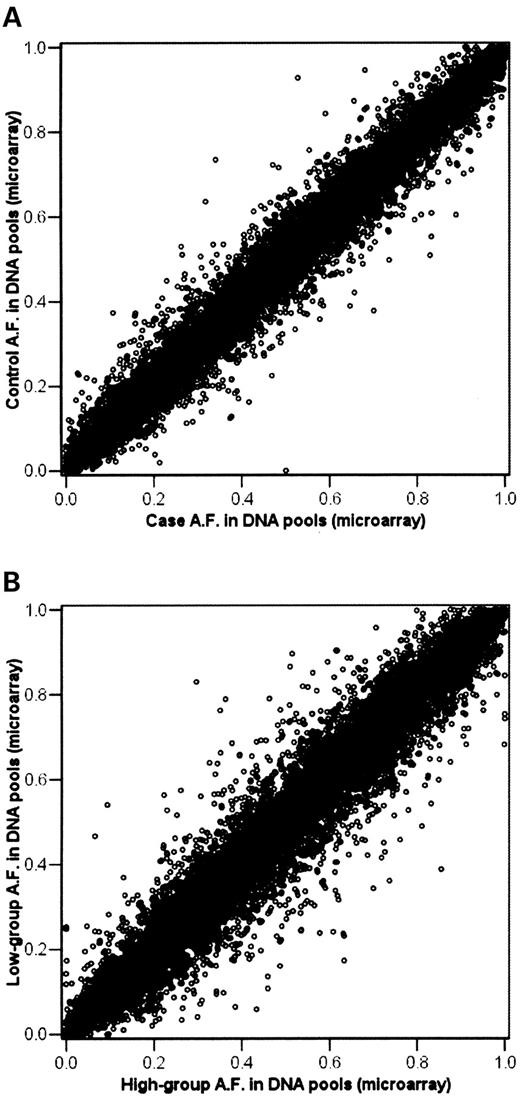
Figure 1. Scatter plots relating SNP-MaP allele frequency estimates for more than 10 000 SNPs for (A) cases versus controls and (B) lows versus highs in two studies. The correlations are 0.984 for cases versus controls and 0.970 for lows versus highs. Bivariate outliers indicate case versus control and low versus high allele frequency differences.
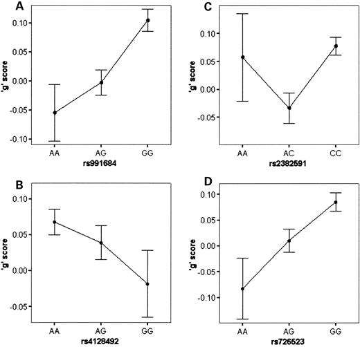
Figure 2. (A–D) Genotype-by-phenotype relationships for individual genotyping results for four significant SNPs. A clear additive effect of genotype on ‘g’ is observed for all but one SNP (rs2382591). The correlation between the genotypes of this SNP and the trait score, however, remains significant. Error bars are +/−1 SEM.
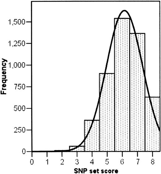
Figure 3. The frequency distribution of ‘SNP-set’ scores for the four SNPs significantly associated with ‘g’. SNP-set scores range from 1 to 8 denoting minimum and maximum summed genotypic scores across the four SNPs. The distribution is mildly skewed (−0.412) because, for all four SNPs, the common allele confers increased ‘g.’.
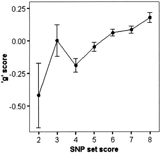
Figure 4. The relationship between ‘SNP-set’ scores and mean standardized ‘g’ scores. The SNP-set scores correlate 0.087 (P=6×10⁻¹⁰, n=4866) with mean standardized ‘g’ scores, accounting for 0.76% of the phenotypic variance. Error bars are ±1 SEM.
Summary of SNP-MaP results for 12 SNPs
| k-Corrected SNP-MaP estimate (SEM) | SNP-MaP differences | |||||||
|---|---|---|---|---|---|---|---|---|
| dbSNP ID | SNP | Allele measured | Cases | Controls | Lows | Highs | Study 1 | Study 2 |
| rs1917126 | G/T | G | 0.523 (0.013) | 0.612 (0.022) | 0.518 (0.011) | 0.601 (0.014) | −0.089 | −0.083 |
| rs745899 | A/T | A | 0.511 (0.031) | 0.664 (0.041) | 0.587 (0.023) | 0.659 (0.009) | −0.153 | −0.072 |
| rs991684 | A/G | A | 0.352 (0.016) | 0.291 (0.016) | 0.346 (0.033) | 0.222 (0.023) | 0.061 | 0.124 |
| rs1343726 | A/T | A | 0.313 (0.018) | 0.221 (0.028) | 0.322 (0.018) | 0.203 (0.035) | 0.092 | 0.119 |
| rs733656 | A/G | A | 0.706 (0.008) | 0.761 (0.015) | 0.714 (0.012) | 0.755 (0.005) | 0.054 | 0.041 |
| rs4128492 | A/G | A | 0.737 (0.017) | 0.791 (0.005) | 0.741 (0.010) | 0.795 (0.012) | −0.054 | −0.054 |
| rs2382591 | A/C | A | 0.206 (0.014) | 0.125 (0.020) | 0.247 (0.021) | 0.157 (0.020) | 0.081 | 0.090 |
| rs2035933 | C/T | C | 0.873 (0.011) | 0.812 (0.014) | 0.903 (0.007) | 0.848 (0.019) | 0.061 | 0.056 |
| rs2254209 | C/G | C | 0.226 (0.011) | 0.142 (0.026) | 0.175 (0.011) | 0.120 (0.014) | 0.083 | 0.054 |
| rs1480952 | C/T | C | 0.294 (0.007) | 0.260 (0.005) | 0.300 (0.009) | 0.224 (0.025) | 0.035 | 0.076 |
| rs726523 | A/G | A | 0.273 (0.013) | 0.218 (0.012) | 0.263 (0.019) | 0.138 (0.024) | 0.055 | 0.125 |
| rs4308066 | A/G | A | 0.810 (0.012) | 0.870 (0.013) | 0.809 (0.012) | 0.865 (0.011) | −0.061 | −0.057 |
Individual genotyping results for four SNPs significantly associated with ‘g’ using the Total Association Model in QTDT analyses
| dbSNP ID | Alleles | Chromosome | χ2 | P-value | n |
|---|---|---|---|---|---|
| rs991684 | A/G | 2 | 10.66 | 0.001 | 5117 |
| rs4128492 | A/G | 6 | 4.12 | 0.042 | 5059 |
| rs2382591 | A/C | 7 | 4.54 | 0.033 | 5151 |
| rs726523 | A/G | 18 | 10.95 | 0.001 | 5172 |
| dbSNP ID | Alleles | Chromosome | χ2 | P-value | n |
|---|---|---|---|---|---|
| rs991684 | A/G | 2 | 10.66 | 0.001 | 5117 |
| rs4128492 | A/G | 6 | 4.12 | 0.042 | 5059 |
| rs2382591 | A/C | 7 | 4.54 | 0.033 | 5151 |
| rs726523 | A/G | 18 | 10.95 | 0.001 | 5172 |
Standardized ‘g’ scores for additive genotypic values for four SNPs significant in QTDT analyses
| SNP | Genotype | Mean score | Standard deviation | N | r | Estimated effect size (%) |
|---|---|---|---|---|---|---|
| rs991684 | AA | −0.055 | 1.01 | 432 | 0.060 | 0.36 |
| AG | −0.003 | 0.991 | 2056 | (P=9.40×10⁻⁶) | ||
| GG | 0.105 | 0.969 | 2629 | |||
| rs4128492 | AA | 0.068 | 0.971 | 2970 | −0.032 | 0.10 |
| AG | 0.039 | 1.011 | 1836 | (P=0.0121) | ||
| GG | −0.019 | 0.958 | 420 | |||
| rs2382591 | AA | 0.057 | 0.979 | 156 | 0.040 | 0.16 |
| AG | −0.034 | 0.996 | 1360 | (P=0.0020) | ||
| GG | 0.077 | 0.978 | 3635 | |||
| rs726523 | AA | −0.083 | 1.003 | 289 | 0.048 | 0.23 |
| AC | 0.01 | 0.97 | 1851 | (P=2.6×10⁻⁴) | ||
| CC | 0.085 | 0.99 | 3032 |
Mean trait scores and correlations between genotype and phenotype were generated using one randomly chosen twin per pair in order to avoid any bias of non-independent sampling. The negative correlation for SNP rs41284924 indicates lower ‘g’ scores for the alphabetically ordered G allele of the A/G SNP.
References
American Psychiatric Association (
Inlow, J.K. and Restifo, L.L. (
Winnepenninckx, B., Rooms, L. and Kooy, R.F. (
Gottfredson, L.S. (
Spinath, F.M., Ronald, A., Harlaar, N., Price, T.S. and Plomin, R. (
Plomin, R., Owen, M.J. and McGuffin, P. (
Butcher, L.M., Meaburn, E., Dale, P.S., Sham, P., Schalkwyk, L., Craig, I.W. and Plomin, R. (
Plomin, R., DeFries, J.C., Craig, I.W. and McGuffin, P. (
Cardon, L.R. and Bell, J. (
Abecasis, G.R., Noguchi, E., Heinzmann, A., Traherne, J.A., Bhattacharyya, S., Leaves, N.I., Anderson, G.G., Zhang, Y., Lench, N.J., Carey, A. et al. (
Kruglyak, L. (
Sham, P.C., Bader, J.S., Craig, I., O'Donovan, M. and Owen, M. (
Barcellos, L.F., Klitz, W., Field, L.L., Tobias, R., Bowcock, A.M., Wilson, R., Nelson, M.P., Nagatomi, J. and Thomson, G. (
Daniels, J., Holmans, P., Plomin, R., McGuffin, P. and Owen, M.J. (
Pacek, P., Sajantila, A. and Syvanen, A.C. (
Plomin, R., Hill, L., Craig, I., McGuffin, P., Purcell, S., Sham, P., Lubinski, D., Thompson, L., Fisher, P.J., Turic, D. et al. (
Germer, S., Higuchi, R. and Higuchi, R. (
Hoogendoorn, B., Norton, N., Kirov, G., Williams, N., Hamshere, M.L., Spurlock, G., Austin, J., Stephens, M.K., Buckland, P.R., Owen, M.J. et al. (
Kirov, G., Stephens, M., Williams, N., Turic, D., McGuffin, P., Plomin, R. and Owen, M.J. (
Norton, N., Williams, N.M., Williams, H.J., Spurlock, G., Kirov, G., Morris, D.W., Hoogendoorn, B., Owen, M.J. and O'Donovan, M.C. (
Olsson, C., Liljedahl, U. and Syvanen, A.C. (
Ross, P., Hall, L. and Haff, L.A. (
Sasaki, T., Tahira, T., Suzuki, A., Higasa, K., Kukita, Y., Baba, S. and Hayashi, K. (
Matsuzaki, H., Loi, H., Dong, S., Tsai, Y.Y., Fang, J., Law, J., Di, X., Liu, W.M., Yang, G., Liu, G. et al. (
Butcher, L.M., Meaburn, E., Liu, L., Hill, L., Al-Chalabi, A., Plomin, R., Schalkwyk, L. and Craig, I.W. (
Hinds, D.A., Seymour, A.B., Durham, L.K., Banerjee, P., Ballinger, D.G., Milos, P.M., Cox, D.R., Thompson, J.F. and Frazer, K.A. (
Trouton, A., Spinath, F.M. and Plomin, R. (
Simpson, C.L., Knight, J., Butcher, L.M., Hansen, V.K., Meaburn, E., Schalkwyk, L.C., Craig, I.W., Powell, J.F., Sham, P.C. and Al Chalabi, A. (
Le Hellard, S., Ballereau, S.J., Visscher, P.M., Torrance, H.S., Pinson, J., Morris, S.W., Thomson, M.L., Semple, C.A., Muir, W.J., Blackwood, D.H. et al. (
Benjamini, Y. and Hochberg, Y. (
Abecasis, G.R., Cardon, L.R. and Cookson, W.O. (
Fulker, D.W., Cherny, S.S., Sham, P.C. and Hewitt, J.K. (
Sham, P.C., Cherny, S.S., Purcell, S. and Hewitt, J. (
Gabriel, S.B., Schaffner, S.F., Nguyen, H., Moore, J.M., Roy, J., Blumenstiel, B., Higgins, J., DeFelice, M., Lochner, A., Faggart, M. et al. (
Barrett, J.C., Fry, B., Maller, J. and Daly, M.J. (
Hardison, R.C. (
De Graeve, F., Smaldone, S., Laub, F., Mlodzik, M., Bhat, M. and Ramirez, F. (
Bartsch, D., Casadio, A., Karl, K.A., Serodio, P. and Kandel, E.R. (
Blanchette, M., Kent, W.J., Riemer, C., Elnitski, L., Smit, A.F.A., Roskin, K.M., Baertsch, R., Rosenbloom, K., Clawson, H., Green, E.D. et al. (
Kato, H., Tjernberg, A., Zhang, W., Krutchinsky, A.N., An, W., Takeuchi, T., Ohtsuki, Y., Sugano, S., de Bruijn, D.R., Chait, B.T. et al. (
Wang, N., Akey, J.M., Zhang, K., Chakraborty, R. and Jin, L. (
Frazer, K.A., Sheehan, J.B., Stokowski, R.P., Chen, X., Hosseini, R., Cheng, J.-F., Fodor, S.P.A., Cox, D. and Patil, N. (
Craig, I.W. and McClay, J. (
Harlaar, N., Butcher, L.M., Meaburn, E., Craig, I.W. and Plomin, R. (
Cohen, J. (
Petrill, S.A., Rempell, J., Oliver, B. and Plomin, R. (
Wechsler, D. (
McCarthy, D. (
Freeman, B., Smith, N., Curtis, C., Huckett, L., Mill, J. and Craig, I. (
Abecasis, G.R., Cherny, S.S., Cookson, W.O. and Cardon, L. (
