Weighted Neighbor Joining: A Likelihood-Based Approach to Distance-Based Phylogeny Reconstruction

Abstract

Introduction

The neighbor joining (NJ) method (Saitou and Nei 1987 ) is widely used to construct large phylogenies because of its elegance and speed, and because when given exact distances, it is guaranteed to reproduce the correct tree. In fact, Atteson (1997) proved that if the distances have very small errors, the correct tree is still obtained, implying that NJ is consistent. Consistency is an important and desirable feature that some other methods (e.g., parsimony and the unweighted pair grouping method with arithmetic means [UPGMA]) lack, but it offers no guarantee of efficiency or of unbiased behavior when the sequences are of finite length.

In maximum-likelihood (ML) phylogeny reconstruction (Felsenstein 1981 ), the effect of a sequence on probabilities at an internal node decays exponentially with distance from that node, making ML trees robust to the presence of distant taxa. For example, one can expect the resolved branches in a primate tree reconstructed by ML to be robust with respect to adding bird or lizard sequences to the data set if the model of evolution is held fixed. Distance-based methods must contend with random errors in the distances that grow exponentially with distance. Because NJ is based on a criterion that does not downweight longer distances, inclusion of different bird or reptile sequences can change the reconstructed branching order of the primates much more easily with NJ than with ML. This has motivated us to create a fast method that, like ML, is inherently robust to the presence of distant taxa.

NJ, like UPGMA before it, consists of two main steps that are repeated until a tree is complete. The first step consists of choosing a pair of taxa to be joined, i.e., replaced by a single new node representing their immediate common ancestor. In the second step, distances from the new node to all other nodes are inferred. Recently, Gascuel (1997) introduced an improvement on NJ called BIONJ, which uses the same first step as NJ, but in the second step uses weighted averages to reduce the variance in the estimates of the new distances. The weights used by BIONJ are based on variances expected for short distances in any evolutionary model.

Criterion for Choosing the Best Pair to Join

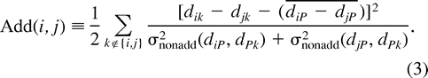
The Weighbor criterion for deciding which pair to join is based on two subcriteria that hold for neighbors (and only for neighbors) when distances are exact. Using the labeling of nodes in figure 1 , with d_ij denoting the distance between nodes i and j, the subcriteria applying to neighbors i and j are:

Additivity:d_ik − d_jkis constant for all choices of a third taxon k.

We call this criterion “additivity” because it will hold if d_ik = d_iP + d_Pk holds for all k (and likewise with j in place of i), with P shown in figure 1 , in which case d_ik − d_jk = d_iP − d_jP.

Positivity:d_ik + d_jl − d_ij − d_kl ≥ 0 for all choices of two other taxa k and l.

This requires the internal branch in the four-taxon tree ((i, j), (k, l)) to have a nonnegative length. That is, d_PQ ≥ 0 in figure 1 . Because Q is defined by k and l, choices of these taxa that give the smallest d_PQ result in the strongest test of this subcriterion.

Due to variations (errors) associated with finite sequence length, estimated distances are not expected to satisfy these criteria in every case in which i and j are neighbors. However, it is possible (using an additional simplifying assumption that the correlations between distances correspond to those for a star phylogeny) to determine the likelihood of the observed distances being generated if the two nodes are in fact sister taxa (i.e., neighbors). Thus, the pair of sequences to be joined at a given step in the procedure may be chosen as the pair for which this likelihood is highest. Estimating the negative log-likelihood gives us a “cost function.” At each stage, we join the pair with the lowest cost, thereby maximizing the probability of a correct join.

Evaluating Additivity

The likelihood that the observed distances are compatible with the additivity criterion for a given pair of taxa i and j is the likelihood that the various d_ik − d_jk values are all estimates of the same thing, d̅_i̅P̅−̅d̅_j̅P̅, where the overbar indicates the optimally weighted average (see appendix 1). Taking the distance errors to be Gaussian gives us a negative log-likelihood of the form

This can be interpreted as a weighted least-squares χ² function; it is also equivalent to a weighted version of the “ThreeTree” criterion of OOta and Saitou (1998) . The variances σ²_nonadd in the denominator consider only “nonadditive” variations and are computed according to

\[\ {\sigma}2nonadd(d_{iP},\ d_{Pk})\ {\equiv}\ {\sigma}^{2}(d_{ik})\ {-}\ {\sigma}^{2}(d_{iP})\ {-}\ {\sigma}^{2}(d_{Pk})\]

(4)

where d_iP and d_Pk are simple estimates given in appendix 1. As discussed in appendix 3, using nonadditive variances in the denominator of equation (3) accounts for the correlations among the distances in the numerator.

Evaluating Positivity

Positivity is defined by an inequality, so the likelihood calculation involves integrating over all amounts by which the inequality could be satisfied. This integral results in the complementary error function erfc(x) defined by (2/

\(\sqrt{{\pi}}\)

⁠)∫^∞_xe−^y2dy. The negative log-likelihood that an instance d_PQ of a Gaussian random variable with variance σ2_PQ comes from a distribution with a positive mean is

The precise definition of d_PQ and the estimation of σ_PQ are discussed below and in appendices 1 and 4; for now, let d_PQ be defined by figure 1 . The log of the error function behaves linearly when |d_PQ| << σ_PQ, and in this situation, Pos(i, j) begins to resemble the linear NJ criterion, although with different coefficients. If the estimated length has a large negative value (d_PQ/σ_PQ << −1), the penalty against joining the pair increases quadratically. If the estimate has a large positive value (d_PQ >> σ_PQ), the function is nearly zero and virtually independent of d_PQ; thus, pairs that clearly obey the positivity criterion are compared on the basis of additivity alone.

Heuristics to Expedite the Best Pair Search

For Weighbor to be useful, it should be much faster than ML on large trees, which implies that it should require no more than order N³ steps. While Add(i, j) can be exactly implemented in an order N³ algorithm by storing N² sums and updating them, the positivity measure entails greater complexity. The most thorough measure of positivity would require evaluating d_PQ for every quartet, which is impossible for an N³ method. This forces us to use certain heuristics to keep the calculation time proportional to N³.

Briefly, for each node i remaining at a given iteration, we first employ a series of pairwise comparisons aimed at finding the node j that is the most likely sister of i. In a comparison between j and j′, we let k = j′ and average over l (l ∉ {i, j, k}) in figure 1 to obtain an estimate of Pos(i, j) − Pos(i, j′). Once the most promising j is found for a given i, the cost function S(i, j) is evaluated for this pair, using an additional heuristic search to find the k and l that cause the worst value of the Pos(i, j) criterion (i.e., minimize d_PQ/σ_PQ). The pair i, j giving the best value of S(i, j) will be the pair that is joined. See www.t10.lanl.gov/billb/weighbor/technical for further details.

These heuristics allow Weighbor to estimate the complete tree in order N³ steps, like NJ and BIONJ. For comparison, the heuristic stepwise addition phase of ML phylogeny methods requires a number of steps proportional to N³L (more precisely, N³L_a, where L_a is the number of nonequivalent columns in the alignment; but in the worst case, L_a = L). Stepwise addition using the method of Fitch and Margoliash (1967) (henceforth “FM”) is order N⁴, while Bulmer’s (1991) generalized least-squares method is N⁶. Distance methods also use an additional order N²L when the distance matrix is computed.

The heuristics we use are not guaranteed to find the optimal pair to join according to the criterion described above. They also can potentially create sensitivity to the order of taxa in the distance matrix. However, as shown below, making use of these heuristics, the method displays performance approaching that of ML and superior to that of existing N³ methods in dealing with long branches.

Calculating Distances to and from the New Node

Once we have decided to join nodes i and j at a new node (called P), there are three kinds of quantities that must be calculated in preparation for the next iteration. The first are the distances from i and j to P; the second are the distances from P to all of the remaining nodes; and the third are variables that will keep track of the variances in the latter distances.

The distance from P to some remaining taxon k ∉ {i, j} is given by the weighted average

where σ²_avg(iP) is the mean squared nonadditivity σ²_nonadd(d_iP, d_Pk) averaged over k. The use of a variance averaged over k was put forward by Gascuel (1997) for BIONJ. It is important that the same weights are used for all k, because this causes errors in d_ij to act as additive errors in later iterations.

The expected error in d_Pk will be greater than (or, if d_iP = 0 or d_jP = 0, equal to) the error expected for an actual sequence at P, because some of the error in d_iP and d_jP is passed on to d_Pk. We keep track of this increased error by introducing a quantity c_P, which is the amount of distance one would add to d_Pk to get the right expected error. These quantities must be included whenever the variance formulas are used, which become

The calculation of the c’s is given in appendix 6, although c_i is zero for any i that is an actual sequence.

Results

We conducted a variety of tests based on sequences generated under the JC model to compare Weighbor with six other methods. The problem of choosing a specific set of trees on which to compare different tree reconstruction methods is complicated by topological biases present in many (possibly all) methods. Once the relative bias between two methods is identified, it is often easy to choose specific trees that will make one method look either better or worse than the other. To avoid this, we consider trees that either explicitly test for bias or are expected to be essentially neutral with respect to bias.

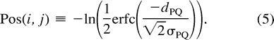
Four-Taxon Star

“Long branches attract” (LBA) is a topological bias toward trees with long branches joined as neighbors (Felsenstein 1978 ). To test for LBA, we simulated four-taxon star phylogenies with two long and two short branches as shown in figure 2 . An unbiased method should choose randomly and equally among the three possible bifurcating topologies. The excess frequency with which the long branches are joined we identify as topological bias (Bruno and Halpern 1999 )

As is well known, parsimony is inconsistent (Felsenstein 1978 ), which implies that for some trees it exhibits maximal topological bias when the sequence length is infinite. In figure 2 , on sequences of length 500, parsimony exhibits a very large bias that increases rapidly with increasing length of the long branches. Both NJ and the PHYLIP implementation of FM (Fitch and Margoliash 1967 ; Felsenstein 1997 ) likewise demonstrate significant, although much smaller, LBA biases that also increase steadily with increasing length of the long branches. The same holds for BIONJ, which is topologically equivalent to NJ on four taxa.

Maximum likelihood (we used fastDNAml [Olsen et al. 1994] ) and Weighbor show no significant bias in these tests, except perhaps for very long branch lengths. Because Weighbor is intended to approximate ML, it is reassuring that the two resemble each other in this test. One might also have expected Weighbor’s bias to be intermediate between the biases of positivity-based methods, such as NJ, and additivity-based methods, such as FM; however, the PHYLIP FM program, called “Fitch,” requires branch lengths to be positive, apparently causing it to have the bias of a positivity-based method. The absence of detectable LBA bias in Weighbor is one good reason for using it.

Based on these bias results, one can predict—and we have confirmed—that parsimony, NJ, and Fitch will perform worse than Weighbor on four-taxon trees with a short internal branch and two long branches that are not joined (this part of the tree space is known as the Felsenstein Zone). Conversely, these biased methods can perform better than Weighbor (and ML!) if the long branches are neighbors in the correct tree and if these branches are of sufficient length.

Trees that obey the molecular clock will tend to favor the LBA bias, because if a clocklike tree has two longest branches, these branches necessarily join. Thus, if real data tend to be clocklike, a biased method could have an advantage. On the other hand, Weighbor gives the correct tree when the distances are exact, suggesting that it is consistent and that if the data are sufficiently convincing, the true tree will be found. Biased methods systematically jump to the conclusion of a clocklike tree (or rather a tree with long branches joined) before the data really support it. Their biases will also tend to result in inflated—and hence misleading—bootstrap values for trees with long branches joined.

Lack of bias alone does not make a method worth using, because choosing a topology at random would also be unbiased by our definition; thus, the ability to find the correct tree when one exists must be tested. In order to avoid any influence of the bias effects we have already tested, we desire test trees that are as neutral as possible with respect to the LBA bias, for example, a four-taxon tree that has all external branch lengths equal. Tests of such symmetric four-taxon trees show negligible differences in performance between Weighbor and the other methods (data not shown), but adding additional taxa to such a tree yields more interesting results.

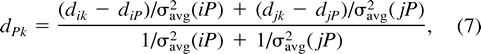
Five-Taxon Tree with a Long External Branch

We consider a symmetric four-taxon tree with a fifth taxon with a longer branch added well away from the short internal branch (fig. 3 ). This tree still avoids effects of the LBA bias (as there is only one long branch), but reveals notable differences among some of the methods. Here we see that three methods, BIONJ, FM, and Weighbor, perform almost as well as maximum likelihood, and these methods are not much affected by the length of the long branch out to a length of 1.0. At lengths beyond 1.0, all methods, including ML, perform progressively worse. This is to be expected due to the difficulty of placing such a distant taxon correctly in the tree.

Clearly, NJ and parsimony begin to feel the effects of the long branch sooner than this. The presence of the long branch interferes with their ability to resolve the short internal branch, even when placement of the long branch itself should not be difficult. When the length of the long branch is 1.0, NJ positions this branch correctly 97% of the time; that is, 97% of the time, the tree reconstructed by NJ has the correct topology or one of the two incorrect topologies obtained by incorrect joins around the short internal branch. ML performs equally well in this regard. This implies that the long branch creates difficulties for NJ not because it is hard to place, but because it causes unnecessary mistakes elsewhere in the tree. We refer to this phenomenon as “long branch distracts” or LBD (not to be confused with similar terminology that was used to describe cases where absence of LBA is disadvantageous [Whiting 1998] ). LBD is caused by a method failing to sufficiently deemphasize the inherently less reliable information contained in longer distances. The existence of the LBD phenomenon has been recognized before (Pollock and Goldstein 1995 ; Gascuel 1997 ) and is partly addressed by the BIONJ program, which successfully avoids LBD in this test.

Parsimony clearly out-performs NJ in this test. It performs worse than the other methods, however. The term LBD may not fully describe parsimony’s difficulty, because when the length of the long branch is 1.0, parsimony positions it correctly only 91% of the time.

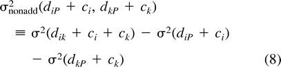
Eight-Taxon Tree with Long Internal Branch

A more stringent test of LBD is shown in figure 4 , where the long branch is now an internal branch. Again, we imposed symmetry on the tree so that LBA bias would not be a factor.

BIONJ is vulnerable to LBD in this case because BIONJ’s joining criterion is no different from NJ’s, and a difficult choice must be made while the long branch is still present. Indeed, for any tree that contains a long internal branch and short internal branches in the subtrees at both ends of the long branch, BIONJ will at some iteration be faced with this problem. We find that BIONJ is only slightly better than NJ in this test, and both methods suffer from LBD: when the long branch had a length b = 0.8, it was positioned correctly 98% of the time by all methods except parsimony (93%), meaning that positioning of the long branch was not the problem.

Parsimony performs quite poorly when the central branch is long, although when this branch is short, parsimony is second only to the likelihood methods. Parsimony’s victories with b = 0.2 over FM, NJ, and BIONJ are statistically significant (P < 0.05), but its advantage over Weighbor is not.

Weighbor performs better than NJ, BIONJ, and, by a small margin, FM over the entire range of distances. At very long distances, Weighbor also performs better than maximum likelihood using the default local search method of FastDNAml for some choices of the input order of taxa (data not shown); with randomized (“jumbled”) input order, FastDNAml is indistinguishable from Weighbor when b = 1.5.

We also investigated how performance varies with sequence length. figure 5 shows results for a tree from figure 4 with an internal branch length b = 1.25. In this figure, Weighbor is about 30% more efficient than parsimony, meaning it can achieve the same accuracy with 30% less data, and is even more efficient relative to NJ and BIONJ. Recall that NJ is consistent, so it will approach 100% correctness with infinite sequence length (when there will be no distance errors); but because NJ does not account for the shape of the error distribution, its efficiency is far from optimal. Everywhere on this plot, Weighbor’s efficiency relative to global ML is at least 90%, and differences between Weighbor and local ML are not statistically significant.

When the long internal branch is reduced to a length of 0.2, all methods perform better and the advantage of using Weighbor is reduced. In this case, Weighbor is about 80% as efficient as local and global ML, 10% more efficient than BIONJ, and 15% more efficient than NJ (data not shown), while differences between Weighbor and parsimony or FM are not significant.

Overall Performance

To summarize, we find that Weighbor is not noticeably influenced by LBA or LBD in our tests. On trees that have only short branches (d ≤ 0.25 in our tests), LBA and LBD are not an issue, and the differences among methods appear minor. However, when long branches are present, more dramatic differences become evident, and Weighbor performs better than all of the methods in our tests except ML.

We know of no examples in which Weighbor is outperformed by NJ or BIONJ, except for trees for which those methods benefit from the LBA bias, and for any such tree, there are always similar trees with different connectivity for which the LBA bias causes the biased methods perform worse (Bruno and Halpern 1999 ). Parsimony performs well on trees with only short branches (d ≤ 0.25), but it performs poorly when long branches (d > 0.5) are present in these tests.

Speed

Weighbor is an order N³ algorithm, and it will run on 256 taxa in about 20 min on a 256-MHz Tatung UltraSparc workstation. Weighbor is about 5 times as fast as parsimony (PHYLIP’s Dnapars; Felsenstein 1989 ) and 200–350 times as fast as FastDNAml using the default local search on sequences of length 500. This factor has only been investigated on up to 64 taxa for FastDNAml but should be relatively independent of the number of taxa; on the other hand, the factor will generally increase with the length of the sequences, although it will also depend on the diversity of the sequences. Weighbor is faster than the order N⁴ Fitch-Margoliash method on 16 or more taxa. Weighbor is substantially slower than both NJ and BIONJ, and the latter could be preferable for very large problems when speed is the primary consideration.

Discussion

By measuring statistical compatibility with the additivity and positivity requirements, Weighbor effectively avoids the LBA bias observed in all of the other methods we tested except ML. Our likelihood-based formalism also results in appropriately less weight being given to long distances, allowing Weighbor to avoid LBD, which clearly affects the performance of NJ and BIONJ. Trees containing two or more distant clades (such as the tree with primates and birds mentioned in the Introduction) are most seriously affected by LBD and stand to benefit most from the use of Weighbor. On trees without distant clades, Weighbor still performs as well as or better than NJ and BIONJ, and Weighbor’s lack of LBA bias is an added benefit. Parsimony performs very well when all the taxa are so closely related that the probability of back substitution is always small, but when one or more long branches are present, parsimony is not a good choice. Based on our tests, Weighbor seems to be a good all-purpose molecular phylogeny reconstruction method for problems for which ML is too slow. Weighbor could also be useful for finding an initial tree which could be further refined by some ML search.

The Weighbor program, including source code, is freely available on the Internet at www.t10.lanl.gov/billb/weighbor or by anonymous ftp at ftp-t10.lanl.gov in pub/billb/weighbor. The sequence length L and the alphabet size β used in calculating variances are adjustable command line parameters. For JC, β = 4, while β < 4 can allow for nucleotide bias or invariant sites, and β > 4 can be used for protein sequences. Generalizing the program to use a more complex model for the function that specifies how variance increases with distance is straightforward. We expect the current version, with appropriate use of the alphabet size parameter (see “parameters” on the webpage), to work well for most molecular applications. Whenever the variance grows rapidly with distance and long branches are present, Weighbor should perform notably better than alternative methods that ignore this variance growth.

In our simulations, the distance matrix was always computed using the correct (JC) model. In real applications, the correct model is unknown, but the best available model should be used to compute the distance matrix, so that the mean nonadditivity will nearly equal zero (Swofford et al. 1996 ; Halpern and Bruno 1998 ). One should also be aware that certain methods for computing distances, notably the K2P (Kimura 1980 ) and Tamura-Nei (1993) formulas, are not very efficient estimators and should be avoided in favor of generalized least-squares (Goldstein and Pollock 1994 ; Pollock 1998 ) or ML distances.

Open in new tabDownload slide

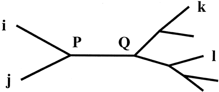
Fig. 1.—Node labeling convention. External nodes i and j are the taxa being evaluated as potential neighbors. Internal nodes P and Q are defined by the tree relating the four taxa i, j, k, and l.

Open in new tabDownload slide

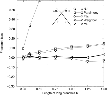
Fig. 2.—LBA bias versus length of long branches. JC sequences of length 500 were simulated on a starlike tree with two short branches of length 0.15 connected to two long branches of length b (see inset). All simulations were repeated 1,000 times. Zero bias implies that each tree is reconstructed in one-third of the repetitions. Plotted is the excess fraction of repetitions in which the long branches are joined. Error bars represent one standard deviation. Fitch refers to the PHYLIP implementation of the FM method, parsimony refers to the Dnapars program in PHYLIP; ML refers to FastDNAml, and Weighbor is the weighted neighbor joining method described here. Distance matrices for all distance methods were computed by the JC formula; infinite distances were replaced by the effectively infinite value of 30.0 changes per site (0.75 − D ≈ 10⁻¹⁸).

Open in new tabDownload slide

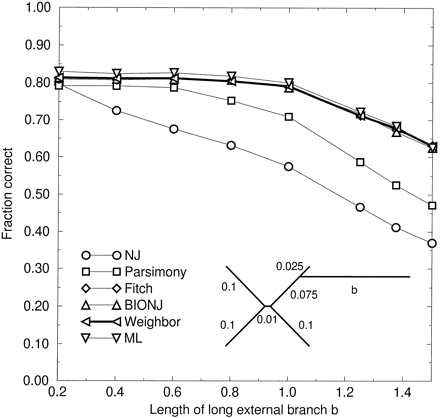
Fig. 3.—Fraction correct versus length of a long external branch. JC sequences of length 500 were simulated on a tree with four branches of length 0.1 connected by an internal branch of length 0.01, and a fifth taxon connected near one tip by a branch of length b (see inset). This figure demonstrates a case of “long branch distracts” (LBD), as does figure 4 . Error bars in this plot and in figure 4 would be ±1.3%–1.6%, or slightly larger than the symbols, as in figure 2 .

Open in new tabDownload slide

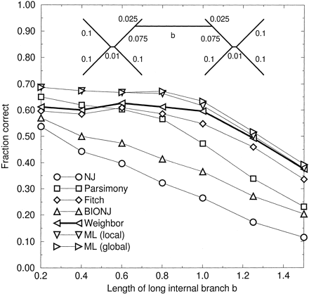
Fig. 4.—Fraction correct versus length of a long internal branch. JC sequences of length 500 were simulated on a tree built from two symmetric trees connected by a branch of length b (see inset). ML (local) is the default search of FastDNAml, and ML (global) is FastDNAml with the more thorough “global” rearrangements option; both methods performed identically in the preceding figures.

Open in new tabDownload slide

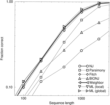
Fig. 5.—Log of fraction correct versus log of sequence length. Sequences of different lengths were simulated on the tree of figure 4 with the length of the central branch b = 1.25.

We thank D. Pollock, J. Thorne, and J. Felsenstein for very useful discussions, the reviewing editor for helpful guidance, and the Santa Fe Institute for facilitating this collaboration. W.J.B. is supported by the DOE Computational Structural Biology initiative through contract W-7405-ENG-36. N.D.S. was supported by Bell Laboratories, Lucent Technologies, and at the Rockefeller University by the National Science Foundation (grant DMR-7932803) and the Alfred P. Sloan Foundation. A.L.H. was supported in part by NIH grant 5P20-RR11830-02 and the Albuquerque High Performance Computing Center.

References