Statistical analysis of fMRI time-series: a critical review of the GLM approach
- Department of Psychology, University of California, Los Angeles, CA, USA
Functional magnetic resonance imaging (fMRI) is one of the most widely used tools to study the neural underpinnings of human cognition. Standard analysis of fMRI data relies on a general linear model (GLM) approach to separate stimulus induced signals from noise. Crucially, this approach relies on a number of assumptions about the data which, for inferences to be valid, must be met. The current paper reviews the GLM approach to analysis of fMRI time-series, focusing in particular on the degree to which such data abides by the assumptions of the GLM framework, and on the methods that have been developed to correct for any violation of those assumptions. Rather than biasing estimates of effect size, the major consequence of non-conformity to the assumptions is to introduce bias into estimates of the variance, thus affecting test statistics, power, and false positive rates. Furthermore, this bias can have pervasive effects on both individual subject and group-level statistics, potentially yielding qualitatively different results across replications, especially after the thresholding procedures commonly used for inference-making.
Introduction
Over the past 20 years the study of human cognition has benefited greatly from innovations in magnetic resonance imaging, in particular the development of techniques to detect physiological markers of neural activity. The most widely used of these techniques capitalizes on the changes in blood flow and oxygenation associated with neural activity (the hemodynamic response), and on the differing magnetic properties of oxygenated and deoxygenated blood. The paramagnetic properties of deoxyhemoglobin (dHb) create local field inhomogeneities, leading to reduced transverse (T2) relaxation times and therefore to a reduction in image intensity. Conversely, increased concentrations of oxyhemoglobin produce increased T2 relaxation times and a relative increase in image intensity. This blood oxygen level-dependent (BOLD) contrast mechanism forms the basis of functional magnetic resonance imaging (fMRI; Ogawa et al., 1990, 1992; Kwong et al., 1992).
While the idea of a hemodynamic response spatially localized to sites of neural activity dates back to Roy and Sherington (1890), the mechanisms by which neural activity triggers changes in cerebral blood volume, flow, and oxygenation are still not fully understood (c.f., Logothetis et al., 2001; Logothetis, 2002) posing a significant constraint on the interpretation of fMRI studies of cognition (Logothetis and Wandell, 2004; Logothetis, 2008). At the level of measurement, the degree to which changes in BOLD signal co-localize with neural activity depends on various imaging parameters, including the magnetic field strength and the imaging sequence used (Ugurbil et al., 2003; Logothetis, 2008). On a more fundamental physiological level, it is also unclear which aspects of neural activity are most closely linked to the hemodynamic response (see Logothetis, 2008, for an excellent overview). While activation of excitatory neurons has been shown to trigger changes in local blood flow (Lee et al., 2010), other studies have reported that input to and activity within local neuronal circuits are both better predictors of the hemodynamic response than output from pyramidal cells (e.g., Logothetis et al., 2001; Goense and Logothetis, 2008), suggesting that the hemodynamic response does not simply reflect the level of spiking activity. Indeed, in some cases the hemodynamic response has been observed in the absence of spiking output (Logothetis et al., 2001; Thomsen et al., 2004; Goense and Logothetis, 2008). A further complication is that both excitatory and inhibitory input create metabolic demands (Buzsáki et al., 2007), making it even harder to interpret the concomitant vascular response as a simple measure of neural firing rate (Logothetis, 2008; although in some cases, neuronal inhibition may produce metabolic and hemodynamic down-regulation; Stefanovic et al., 2004). Overall, the hemodynamic response is likely to reflect an average response to a range of metabolic demands imposed by neural activity, including both excitatory and inhibitory post-synaptic processing, neuronal spiking, as well as neuromodulation (Logothetis, 2008; Palmer, 2010).
Bearing these caveats in mind, the reminder of the paper will focus on statistical methods for separating noise from systematic fluctuations of the BOLD signal induced by experimental stimulation. Following a brief review of the general linear model (GLM) framework, the paper will focus on the degree by which single-subject fMRI time-series conform to the assumptions of the framework, and on the approaches used to mitigate infringements of these assumptions. Finally, the paper will also discuss methods to combine datasets from multiple subjects, with respect to their inferential scope and validity.
For clarity, the rest of the manuscript will use the term “volume” to refer to an individual data acquisition point, typically a three dimensional image of the MRI signal at multiple points throughout the brain acquired over the course of several seconds. Multiple volumes acquired as one continuous stream of data are referred to as a “run” or “scan.” Each subject usually undergoes multiple runs, sometimes with brief interruptions in between, but usually whilst remaining inside the bore of the magnet. A set of multiple runs is referred to as a “session.” A standard fMRI dataset for a complete experiment usually consists of one (or more) session from each of a number of subjects.
Single-Subject Analysis (I): The General Linear Model Approach
An fMRI dataset, can be seen as a set of cuboid elements (i.e., voxels) of variable dimension, each of which has an associated time-series of as many time-points as volumes acquired per session. The aim of a (conventional) statistical analysis is to determine which voxels have a time-course that correlates with some known pattern of stimulation or experimental manipulation. The first step in fMRI data analysis is to apply a series of “pre-processing” transformations with the aim of correcting for several potential artifacts introduced at data acquisition. Each transformation can be applied as required depending on the specific experimental design or acquisition protocol. The most typical steps include adjusting for differences in the acquisition time of individual image slices, correction for subject motion, warping individual subjects data into a common space (“normalization”), and temporal and spatial smoothing (see Jezzard et al., 2002). Following pre-processing, data analysis is often carried in two steps: a separate first-level analysis of data from each individual subject, followed by a second-level analysis in which results from multiple subjects are combined.
In the GLM approach, the time-course associated with each voxel is modeled as a weighted sum of one or more known predictor variables (e.g., the onset and offset of an experimental condition) plus an error term. The aim of the analysis is to estimate if, and to what extent, each predictor contributes to the variability observed in the voxel’s time-course. Consider, for example, an experiment in which the BOLD response, y, is sampled n times (i.e., volumes). The intensity of the BOLD signal at each observation (yi) can be modeled as the sum of a number of known predictor variables (x1…xp) each scaled by a parameter (β):
The aim of the first-level statistical analysis is to determine how large the contribution of each predictor variable xi is to the observed values of y. That is to say, how large each scaling parameter βi is, and whether it is significantly different from zero. Using the more compact matrix notation, the GLM can be re-expressed, in its simplest formulation, as:

Where Y is an n × 1 column vector (i.e., n rows, 1 column) representing the BOLD signal time-series associated with a single voxel. X is the n × p design matrix, with each column representing a different predictor variable. Of interest are the columns representing manipulations or experimental conditions, although the matrix typically also includes regressors of non-interest, modeling nuisance variables such as low-frequency drifts and motion. β is the p × 1 vector of unknown weights setting the magnitude and direction of the (unique) association between each given predictor variable and the data Y. Finally, ε is an n × 1 vector containing the error values associated with each observation (i.e., the value of each observation that is not explained by the weighted sum of predictor variables).
Figure 1 depicts the GLM model for an imaginary voxel with associated time-series Y, as the linear combination of three regressors of interest (e.g., tasks A,B,C) and a number of nuisance variables (here six motion regressors and a linear drift), each scaled by a vector of unknown amplitudes (β), plus an error term ε.
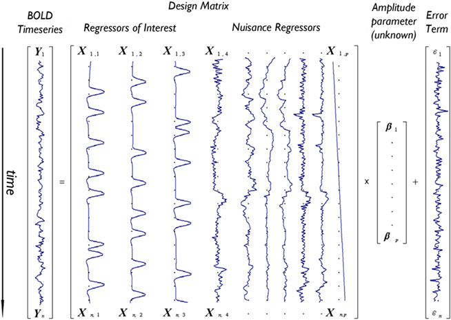
Figure 1. Depiction of the GLM model for an imaginary voxel with time-series Y predicted by a design matrix X including 10 effects (three regressors of interest – e.g., tasks A,B,C – and seven nuisance regressors – e.g., six motion parameters and one linear drift) of unknown amplitude βi, and an error term.
The standard approach to fMRI analysis is to fit the same model independently to the time-course of each voxel. Spatial covariance between neighboring voxels is thus typically ignored at the model fitting stage. The presence of more response variables (i.e., voxels) than observations (i.e., volumes), together with the aim of making topographically specific claims about BOLD activity, has traditionally motivated this “massive-univariate” approach. Recently, however, a lot of effort has gone into developing multivariate techniques to address the question of what information specific brain areas represent (as opposed to the “localizationalist” approach typical of univariate analysis; c.f., Kriegeskorte et al., 2006, 2008; Bowman, 2007; Bowman et al., 2007).
Several methods are available to estimate the value of the unknown parameter β, and therefore assess whether a given predictor variable significantly explains some portion of the variance observed in a voxel’s time-course, including the ordinary least squares (OLS), (feasible) generalized least squares (GLS), and the so-called Smoothing and “Sandwich” approaches (see Waldorp, 2009, for a clear overview of these methods). In its simplest OLS form, the optimal parameters are defined as those that minimize the sum of squared residuals1:  (i.e., the squared difference between the observed signal Y and the expected signal as specified by the X matrix scaled by the β parameters). The unknown parameter and its variance are thus estimated as follows2:


According to the Gauss–Markov (𝒢𝓜) theorem, the OLS will correspond to the best linear unbiased estimator (BLUE) of the population parameters, in the class of unbiased estimators, provided the following assumptions relating to the properties of the error term and the parameters hold true3:
(A1) Errors are independently and identically distributed (i.i.d.) ∼N(0, σ2I)
(A2) he regressors in the X matrix are independent of error [i.e., E(ε,X) = 0], non-stochastic (i.e., deterministic), and known.
(A3) No regressor is a linear transformation of one (or more) other regressors.
It should be noted that (A1) is in fact a three-part assumption requiring that (A1a) the errors for different observations (time-points) are not correlated [i.e., Cov(εi,εj) = 0]; (A1b) the expected value of the error term is zero [i.e., E(ε) = 0]; and (A1c) the variance of the error is σ2 at all observations.
Crucially, a statistical model is only valid inasmuch as its assumptions are met. When this is not the case, inferences drawn from it will be biased and can even be rendered invalid. The reminder of this paper focuses on the degree to which fMRI data abide by the above assumptions, the consequences of their infringement, and describes the main methods currently available to adjust for such situations.
Single-Subject Analysis (II): The 𝒢𝓜 Assumptions and fMRI Time-Series
Autocorrelation
One major potential violation of the model’s assumptions arises from the fact that fMRI data represent a time-series. In particular, correlations between residuals at successive time-points can violate the i.i.d. assumption (A1a). Common sources of noise that can introduce serial correlations include hardware related low-frequency drifts, oscillatory noise related to respiration and cardiac pulsation, and residual movement artifacts not accounted for by image registration (c.f., Weisskoff et al., 1993; Friston et al., 1994; Boynton et al., 1996). The presence of serial correlation does not directly affect unbiasedness of the  , but can produce biased estimates of the error variance. This can in turn lead to biased test statistics (e.g., t or F values), and affect statistical inferences based on those statistics.
In fMRI data, the problem is typically one of systematically over-estimating the error degrees of freedom, since the presence of serial correlations means that the true number of independent observations (the effective degrees of freedom) will be lower than the apparent number of observations. In turn, this produces an underestimate of the error variance and thus an inflated test statistics (since the error variance is included in its denominator). The artificially liberal nature of inferences drawn in the absence of correction for autocorrelation was demonstrated by Purdon and Weisskoff (1998) who found false positive rates as high as 0.16 could occur for a nominal α-level of 0.05. Several different approaches have been suggested to minimize this problem.
Temporal smoothing (“pre-coloring”)
Friston et al. (1995) and Worsley and Friston (1995) suggest an extension of the GLM to accommodate serial correlation via “temporal smoothing.” Their proposal is to re-frame (1) as:

where Σ represents some process hidden in the residual characterizing the serial correlation, and ε represents a “well-behaved” error term ∼N(0, σ2I). By then imposing a linear transformation S to (4) the idea is to “swamp” and thereby minimize the endogenous – unknown – correlation structure with some exogenously imposed, therefore known, correlation structure S, obtaining:

The assumption underlying this method is that the S transformation is robust enough so that SΣST∼SST, thereby effectively “swamping” the unknown endogenous serial correlation. If this assumption holds, the “colored” noise is identically distributed ∼N(0, σ2ST) (Friston et al., 1995). The derived β-estimates remain unbiased but do not retain maximal efficiency, thus degrading power, as a function of how (in)effectively the endogenous correlation is swamped. In addition, the pre-coloring smoothing function acts as a low-pass filter, and may risk attenuating experimentally induced signals of interest (Marchini and Ripley, 2000; Woolrich et al., 2001). Partly as a response to these problems, the pre-coloring approach has now been largely superseded by the pre-whitening approach.
Pre-whitening
Rather than attempting to mask an unknown covariance structure with a known one, the pre-whitening strategy attempts to estimate and remove the autocorrelation prior to estimating the model parameters (Bullmore et al., 1996). This technique makes use of a two-pass procedure. In the first pass, a GLM is fit to the data under the infringed i.i.d. error assumption. The residuals derived from this model are then used to estimate the autocorrelation structure actually present. The autocorrelation is then modeled with a simple Auto-Regressive model of order 1 [AR(1)], in which the error at each time-point is assumed to be a combination of the error at the previous time-point and some “fresh” error. Once the parameters for this model have been estimated, the raw data is “pre-whitened” by removing the estimated covariance structure. Finally, a second pass of the GLM estimation is carried out on the whitened data. The intuition underlying such an approach is that if a good estimate of the autocorrelation structure can be obtained and removed from the data, the i.i.d. assumption (A1a) will hold. As a parallel to (5), this approach can be expressed as:

where K ≈ Σ. Thus, instead of the convolution with a temporal smoothing matrix S as in Friston et al. (1995), the pre-whitening approach uses a de-convolution matrix obtained by data driven estimation of the Σ structure. Unlike the pre-coloring approach, pre-whitening also has the advantage that the resulting parameter estimates will be the BLUEs. Thus, equations (2) and (3) can be re-written as:
If the process Σ is exactly characterized by K, then in the transformed data the error variance is equal to σ2I again. Compared with pre-coloring, pre-whitening has the advantage of being more efficient (Woolrich et al., 2001) across different experimental designs, and particularly for rapid event-related designs where much of the experimentally induced signal is concentrated in high temporal frequencies. The approach, however, relies heavily on accurately characterizing the endogenous correlation structure and non- optimal modeling can reduce efficiency and induce significant bias, affecting the magnitude of test statistics (Friston et al., 2000a). In response to these problems, several authors have suggested the use of more complex models allowing for serial correlations over longer periods of time (Worsley et al., 2002), greater flexibility in the local noise modeling (e.g., Locascio et al., 1997; Purdon et al., 2001), and non-parametric approaches (Woolrich et al., 2001).
Lenoski et al. (2008) compared the performance of several different strategies for whitening residuals, including the global linearized AR(1) algorithm implemented in SPM2/5 (Frackowiak et al., 2004), a regularized non-parametric correction (Woolrich et al., 2001) similar to the one implemented in FSL (Smith et al., 2004), and a voxel-wise, regularized AR(m) autocorrelation algorithm (Worsley et al., 2002) as implemented in fMRIStat. Across six algorithms, the global linearized AR(1) model proved to be the least effective, decreasing the count of non-white residuals to about 47%. Notably, the algorithm was effective at eliminating positive autocorrelation structures. Due to the inflexibility of the global approach, in which the same, positive correlation structure is assumed to exist at every voxel, white and negative autocorrelations were poorly modeled. As a consequence, this approach induced negative correlations that were not originally in the data (the practical implications of this remain debatable however, as Lenoski et al. (2008) also report that positive autocorrelations are present in the overwhelming majority of voxels; see also Woolrich et al., 2001; Worsley et al., 2002). Regularized algorithms, including AR(1) and non-parametric methods, successfully reduced non-whitened residuals to about 41 and 37% of the total voxels. As with the global linearized AR(1) approach, positive correlations were greatly reduced, although there was again a slight increase in negative correlations. The best performance was obtained with non-regularized non-parametric and AR(2) algorithms, which decreased the number of non-white residuals to an average of 1.6 and 0.5%, respectively. Overall, this supports the idea that the major source of autocorrelation in BOLD time-series is successfully captured by an AR(2) model.
Explicit noise modeling
Finally, an alternative approach to the data driven estimation of serial correlation has been proposed by Lund et al. (2006). In their interpretation, autocorrelation amongst residuals can often be taken as evidence of unmodeled, but potentially known, sources of variance. In their “nuisance variable regression” (NVR) approach they attempt to explicitly model within the design matrix several factors believed to induce autocorrelation, including hardware related low-frequency drift, residual movement effects, and aliased physiological noise (i.e., cardiac pulsation and respiration; see also Lund et al., 2006). Empirical tests suggested that the approach is effective in capturing the modeled sources of noise such as cardiac and respiratory effects (see also Razavi et al., 2003). Indeed, the NVR approach resulted superior to both the AR(1) and the simple high-pass filtering approaches for dealing with serial correlation. However, despite the potential appeal of this approach, it is highly dependent on the sources of noise being well characterized, and will still require some form of data cleaning to account for additional unmodeled sources of temporal correlation.
Heteroscedasticity
Assumption (A1c) requires the variance of residuals to be constant across observations (i.e., time-points), and the covariances (i.e., the off-diagonal elements of the variance–covariance matrix) to be all equal to zero [i.e., var(ε) = σ2I]. Violation of such assumption is referred to as heteroscedasticity. When this assumption is not upheld the estimator ( ) is still unbiased, but no longer efficient, usually resulting in confidence intervals that are either too wide or too narrow. As for the case of autocorrelation, if the variance is biased subsequent parametric testing will yield incorrect statistics. In the fMRI literature heteroscedasticity has received relatively little attention. As a notable exception, Luo and Nichols (2002, 2003) discuss the possibility of heteroscedasticity in fMRI data, for example due to a dependency of the variances on the response, or because of other factors such as time or physical ordering (in Luo and Nichols, 2002, violations of homoschedasticity are indeed found, mostly due to artifacts).4
Multicollinearity and X Matrix Mis-Specification
Multicollinearity
Assumption (A3) requires that none of the explanatory variables (i.e., columns of the X matrix) is perfectly correlated with any other explanatory variable, or any linear combination of. In the presence of perfect multicollinearity the X matrix is rank- deficient, the inverse of (XTX) does not exist, and infinite solutions equally satisfy the GLM system of equations. In reality, however, the problem with multicollinearity is one of degree. The impact of multicollinearity on the β-estimates of the correlated columns is to reduce their efficiency (i.e., increase  ) as a positive function of the degree of collinearity present. The fundamental problem is that as two columns become more and more correlated it becomes impossible to disentangle the unique impact of each on the dependent measure. The confidence intervals for the coefficients thus become wide, possibly including zero, making it difficult to assess whether an increase in a regressors is associated with a positive or negative change in the dependent measure (i.e., Y). The consequence of this issue is then a strong bias in the inferential statistics (e.g., t-test – which can be either positive or negative). It should be noted, however, that multicollinearity only affects the repartition of variance among the individual regressors. Overall model statistics such as R2 and the significance of the model remain unaffected, possibly leading to the seemingly paradoxical situation where individual βs have low significance but the overall model fit is high. A clear example of the impact of multicollinearity in functional neuroimaging experiments is provided in Andrade et al. (1999), where, in a PET experiment, the activations associated with a given regressor in the presence, or absence, of a strongly covarying second effect are qualitatively different. As the authors remark, the results obtained from the correlated and uncorrelated models could lead to qualitatively different conclusions (Andrade et al., 1999). Overall, this example shows that in the presence of multicollinearity functional neuroimaging results can be misleading and misinterpreted.
As for the homoscedasticity assumption, the multicollinearity issue did not find, so far, much space in the fMRI methodology literature. There may be at least two reasons for this: first, the standard use of the pseudo-inverse method; second, this problem is typically dealt with at the creation of the experimental design (i.e., the X matrix). Indeed, much more energy has been spent on the issue of design efficiency (including multicollinearity minimization; c.f., Dale, 1999; Wager and Smith, 2003; Henson, 2007; Smith et al., 2007).
X matrix mis-specification (I): model building
Mis-characterizing the expected BOLD signal, by mis-modeling the X matrix, can be an important source of error. According to Petersson et al. (1999), the specification of the X matrix faces two connected trade-offs related to the cases of over- and under- specification. On the one hand, inclusion of a maximum number of effects in the model would be desirable to increase fit, though at the cost of reducing power (by consuming one df for each additional effect), while the marginal increase of explained variance decreases with each additional factor. Further, over-modeling of the signal may degrade the generalizability of the results. On the other hand, exclusion of relevant factors from the model may have the effect of inflating the error variance, reducing power, and possibly introducing serial dependencies in the error term, thus infringing assumption (A1a). At the same time, however, exclusion of irrelevant effects from the model has the (positive) consequence of increasing power via increase of the dfmodel (one per each excluded variable; see Petersson et al., 1999, pp. 1246–1247 for a complete discussion on the point).
Overall, the consequences of even minor cases of mis-modeling, can result in severe loss of statistical power and inflation of the false positive rate far beyond the nominal α-level (Loh et al., 2008). Along similar lines, Razavi et al. (2003) analyze the importance of model building with respect to the impact of model mis-specification (by either excluding appropriate effects or including inappropriate effects) on its goodness of fit and validity. Using a forward selection approach, inclusion of appropriate regressors (e.g., task and several noise sources) increased both statistics. Inclusion of an inappropriate term, on the other hand, increased the model goodness of fit, but strongly decreased the model validity. Finally, the authors also point out that the sheer number of activated voxels under each model, a heuristic often used for model selection, was often in conflict with model validity and goodness of fit statistics. In particular, inclusion of an inappropriate effect in the model reduced its validity, but increased the number of active voxels.
X matrix mis-specification (II): the hemodynamic response function
Once the X matrix is properly specified, the regressors are typically convolved with a hemodynamic response function (HRF), in order to transform neural responses to on–off stimulation into an expected vascular signal (see Boynton et al., 1996). The HRF thus characterizes the input–output behavior of the system (Stephan et al., 2004), imposing an expectation on how the BOLD signal in a voxel should vary in response to a stimulus. Even for a well specified X matrix, incorrect modeling of the HRF might cause significant discrepancy between the expected and the observed BOLD signal, increasing the variance of the GLM coefficients, degrading power, and decreasing the model validity (c.f., Aguirre et al., 1998; Loh et al., 2008; Waldorp, 2009). Indeed, even minor model mis-specification can result in substantial power loss and bias, possibly inflating Type I errors (Lindquist et al., 2009). It is then all the more problematic that the HRF is known to be highly variable across individuals, and, within individuals, across tasks, regions of the brain, and different days (Aguirre et al., 1998; Handwerker et al., 2004). The input–output relationship between stimulation and BOLD response can be modeled in one of several ways. The most typical approach is to assume a linear time-invariant system, where the HRF is modeled by a set of smooth functions that, when overlapping, add up linearly (Friston et al., 1994; Boynton et al., 1996). In this approach, many models have been proposed, with various degrees of flexibility. At the low end of the spectrum, the HRF is considered to have a fixed shape (e.g., the difference between two gamma functions) except for its amplitude (Worsley and Friston, 1995). A popular alternative is to employ a canonical HRF together with two derivatives, to allow for (small) variations in latency and dispersion (Friston et al., 1998). Even greater flexibility can be afforded by using a larger set of basis functions, typically constrained to the space of plausible HRF shapes (Woolrich et al., 2004; Penny and Holmes, 2007) and its relevant parameters (Liao et al., 2002). At the top end of the flexibility spectrum, finite impulse response (FIR) basis sets allow estimation of the height of the BOLD response at each time-point (Glover, 1999; Ollinger et al., 2001).
In general, inclusion of multiple parameters has the advantage of acknowledging and allowing for known HRF variability, thus increasing sensitivity (Woolrich et al., 2004). At the same time, however, the increased flexibility comes at the cost of potentially fitting physiologically ambiguous or implausible shapes (Calhoun et al., 2004; Woolrich et al., 2004), fewer degrees of freedom, and decreased power (Lindquist et al., 2009). Furthermore, when multiple HRF shapes are tested, it is not clear how to aggregate the results for group-level analysis (c.f., Calhoun et al., 2004; Steffener et al., 2010), nor it is clear how to interpret differences between tasks when spread over a multitude of parameters (Lindquist et al., 2009). A different approach is to adopt physiologically informed models of BOLD response, such as the Balloon model (Buxton et al., 1998; Friston et al., 2000b). In this model, a set of differential equations specifies a dynamic link between neuronal activity and transient increases in the rate of cerebral blood flow, in terms of volume and dHb content. The elicited BOLD signal is then considered to be proportional to the ratio of these two quantities (Friston et al., 2000b). While more biologically plausible, this approach face several difficulties relating to estimation of a large number of parameters, unreliability of estimates in the presence of noisy data, and the lack of a direct framework for inference-making (Lindquist, 2008).
Overall, most cognitive fMRI research to date appears to be exclusively focused on estimating the magnitude of evoked activations (Lindquist and Wager, 2007; Lindquist et al., 2009), and does not pay much attention to HRF variability. Indeed, as revealed by a recent survey of 170 fMRI studies, 96% of experiments adopting an event-related design used a canonical HRF model, thus ignoring differences in shape between individuals or areas of the brain (Grinband et al., 2008). As noted by Lindquist (2008), building of more sophisticated HRF models is likely to be, in the coming years, one of the areas of great multidisciplinary focus.
Linearity
The GLM approach also assumes effects to add linearly to compose the response measurements. Boynton et al. (1996) tested this assumption by parametrically varying a visual stimulus’ duration and contrast. Investigating the additivity of the noise in V1, they concluded that although deviations from linearity were measurable, these were not strong enough to reject the GLM. Support for the use of a linear approach was also offered in Cohen (1997), where response amplitudes to parametric variations of the stimuli were well modeled by a piecewise linear approximation. Despite this initial evidence, it has now been extensively shown that there are at least two sources of non-linearities in the BOLD signal: the vascular response, especially the vasoelastic properties of the blood vessels (see Buxton et al., 1998), and adaptive behavior in neuronal-response (e.g., Logothetis, 2003).
Vazquez and Noll (1998) tested the linearity of the BOLD response to (visual) stimulation of varying length. Under the linearity assumption, it should be possible to predict the amplitude of the response at a given duration by multiplying the amplitude of the response at a shorter duration an appropriate number of times. When stimuli of at least 5 s were used to predict the BOLD response amplitude at longer intervals, this expectation was met. However, when stimuli of 4 s or less were used to predict the response at longer durations, these were found to greatly overestimate the observed amplitudes. A similar result was reported, using auditory stimuli, by Robson et al. (1998). Consistently with the results in Vazquez and Noll (1998), it was possible to predict the BOLD response amplitude at long durations with stimuli of at least 6 s. Stimuli of shorter duration yield dramatic overestimates of the response amplitude at longer durations, as a positive function of the time difference between the predictor and the predicted stimulus length (see Robson et al., 1998, Figure 4, p. 191). The authors thus suggest including in the model an adaptive component that may discount the response amplitude for short stimulations specified as:

Equation (7) essentially represents a scaling factor to be applied to the amplitudes of short latency stimuli in order to correct for “transient” non-linearity. In Robson et al. (1998), this approach reduced the discrepancy between the observed response at the longest latency (25.5 s) and the predicted one (from the shortest latency – 100 ms) from 11.09% signal change to only 0.88%.5
Friston et al. (1998) used parametric variations in the rate of word presentation to assess the presence of non-linear BOLD effects. The observed departure from linearity was interpreted in terms of a hemodynamic “refractoriness,” according to which a prior stimulus interacts with a following – temporally contiguous – stimulus by modulating its response amplitude. As a solution, the authors proposed “linearizing the problem,” by employing Volterra series to overtly characterize the non-linear component of the response. The observed BOLD signal Y(t) can then be modeled as:

The second term of the equation represents the change in output (i.e., Y) for a given change in input. The third term is the part of the model that describes the effect of the response at one time-point on a temporally contiguous time-point, with the parameters g0, g1, g2 representing the scaling factor of a series of P basis functions approximating the zeroth, first, and second Volterra smoothing kernels (see Friston et al., 1998, p. 42). One criticism to this approach raised in Calvisi et al. (2004) and Friston et al. (2000b) is that while data driven computation of Volterra series parameters may allow for a better input–output mapping, it does so in a black-box fashion without being informative on what are the processes generating the non-linearities. In response to these criticisms Friston et al. (2000b) present evidence for the non-linearities expressed in the Balloon model of hemodynamic signal transduction (see Buxton et al., 1998) being compatible with a second order Volterra characterization, thus adding biological plausibility to the model.
A different approach has been proposed by Wager et al. (2005) who report substantial non-linearities in the magnitude, peak delay, and dispersion of the response for a stimulus presentation rate of 1 s. Noting the consistency of such non-linearities across the brain they suggest empirically deriving the functional form of each of these characteristics of the response as a function of stimulus history. The authors approximate the non-linearities with a biexponential model:
y = Ae−αX + Be−βX
By fitting the parameters A and α, B and β, the scaling and exponent of two exponential curves, the authors empirically characterize the non-linear changes in BOLD magnitude, onset time, and peak delay. The idea is to first run an experiment from which to derive the fixed parameters estimates and then use the non-linear characterizations as scaling factors for individual responses – according to the history of stimulation up to each response – in following experiments.
The issue of non-linearity is particularly relevant to fast event-related designs. When short intervals separate periods of stimulation, the response to the individual stimuli will superpose, and will do so sub-additively, reducing the observed signal, presumably as a consequence of neuronal and vascular factors (e.g., Birn and Bandettini, 2005; Heckman et al., 2007; Zhang et al., 2008). Several studies have now documented the decrease in the estimated response amplitude at short inter-stimulus intervals (ISI). In Miezin et al. (2000), for example, average ISIs of about 5 s (with a minimum of 2.5 s) resulted in a decrease of 17–25% of the signal obtained in widely spaced trials (e.g., 20 s). Similarly, Zhang et al. (2008) reported significant decreases in response amplitude for ISIs of 1 and 2 s, as compared to longer spacing (i.e., 4, 6, and 8 s). At the lower end of stimulus spacing, Heckman et al. (2007) compared BOLD response in visual cortex to stimuli of varying contrast under a “spaced” (3 s ISI) and a rapid (1 s ISI) presentation. Qualitatively, the patterns of response across designs were similar. Quantitatively, however, the rapid presentation had the effect of scaling the strength of the response. In particular, the response reduction observed when switching from a spaced to a rapid presentation was found to be similar to the reduction observed when decreasing the stimulus contrast (under the same presentation condition). In primary visual cortex, for example, switching to a rapid design induced a response reduction equivalent to that observed when decreasing the stimulus contrast by 84%. Finally, while the response non-linearity appears stable within a given region (Miezin et al., 2000), it may vary greatly across different primary cortices (e.g., Miezin et al., 2000; Soltysik et al., 2004) and may increase in associative areas (Huettel and McCarthy, 2001; Boynton and Finney, 2003; Heckman et al., 2007).
Overall, as noted by Wager et al. (2005) non-linearities are largely ignored in the neuroscientific and psychological BOLD-fMRI literature. Several reasons may underlie this observation. First, there exists an “envelope” within which the linearity assumption holds (e.g., ISIs ≥ ∼4 s). An informal PubMed survey of 20 papers published in 2010 mentioning the words “rapid/fast event-related fMRI” in the abstract revealed that half the designs used an average ISI of at least 4 s. Of the remaining, half the designs made use of an ISI between 3.5 and 4 s, and the remaining employed even shorter intervals. The large majority of studies thus falls at the boundary of the envelop, or well within it. No single study mentioned non-linearities in BOLD response at short ISIs. All studies except for one, however, made use of stimuli (pseudo-)randomization and/or ISI random jittering, with the aim of maximizing power and mitigating non-linear effects by making each stimulus category equiprobable at each trial (c.f., Dale, 1999; Henson, 2007). Second, the increased statistical power conferred by a greater number of trials, under fast designs, may well outweigh the amplitude reduction induced by overlapping BOLD responses (calculated to be about 20% in Miezin et al., 2000). Third, the bulk of the work has been devoted to determining canonical responses to a single stimulus rather than to exploring interactions among multiple stimuli. Finally, most proposed solutions (e.g., Volterra series; see Friston et al., 1998, 2000a) require fitting of a large number of parameters which may cause severe degradation of power.
Multiple Subjects Analysis
Once single-subject data has been analyzed for a set of participants, individual results are aggregated to assess commonality and stability of effects within or across groups of interest (Holmes and Friston, 1998; Worsley et al., 2002). Prior to group analysis, however, for datasets to be comparable across subject, individual results are warped into a common reference space (typically either the Talairach, Talairach and Tournoux, 1988, or the MNI152, Evans et al., 1997), in order to “align” corresponding cerebral structures across subjects with differing brain anatomy. This normalization procedure is all but uncontroversial, especially in relation to its effectiveness (see Brett et al., 2002), however, a discussion of the issue extends beyond the scope of this review.
One of the central issues in group analysis concerns the scope of the inferences one may validly draw from aggregate statistics. As will be discussed below, some group analysis strategies only afford making valid inferences about the specific sample (i.e., participants) one has tested. Other strategies, however, afford making valid, and typically more interesting, inferences about the population from which the sample was drawn.
Fixed Effects
As Holmes and Friston (1998) nicely put, classical statistical hypothesis testing proceeds by comparing the difference between the observed and hypothesized effect against the “yardstick” of variance (p. S745). The scope of an inference is then bound by the yardstick employed. In a fixed effects (FFX) analysis, the variance considered is that derived from scan-to-scan measurement error, and represents the within-subject variability ( ). This variability may include physiological task-related (e.g., adaptation, learning, and strategic changes in cognitive or sensory-motor processing) and task non-related effects (e.g., changes in global perfusion secondary to vasopressin secretion in the supine position), as well as non-physiological noise, such as gradient instabilities (c.f., Friston et al., 1999a). In this approach statistical testing assesses whether a response is significant with respect to the precision with which it can be measured (Friston et al., 2005). Paraphrasing the very intuitive example offered in Mumford and Nichols (2009), if one were to measure the length of hair from the same set of participants twice, it is reasonable to assume that the only difference across the two measurements should relate to small variation around the average hair length of each participant. In this sense, for each subject the magnitude of the effect is considered to be fixed. FFX analyses thus represent the population variance as being a sole function of within-subject variability divided by the product of subjects (N) and number of observations per subject (n) (c.f., Penny and Holmes, 2007). For a given subject i, the observed response in trial j (i.e., yij) is modeled as varying around the subject’s mean effect di plus a within-error component eij (with mean zero and variance
  ):
):

For a single subject i, then, the (maximum likelihood) parameter estimate and its variance are:


As shown in equation (11), the variance of the effect for each subject i is the within-error divided by the number of observations n. To compute the group-level analysis of the population effect (dpop), then, it suffices to aggregate the individuals’ effects ( ) for all N subjects, yielding (see Penny and Holmes, 2007, Section 3 for the full derivation):


The crucial point shown in (13) is that the group estimate’s variance in an FFX approach is a function of the scan-to-scan (i.e., within-subject) variability  only. This group analysis is thus conceptually equivalent to concatenating all data and performing a single GLM on a “super-subject” with N × n observations.
Importantly, the inferences drawn from a FFX analysis are not invalid, rather they are only valid with respect to the yardstick employed (i.e.,  ). Inferences are thus supported at the level of the sample analyzed, but not at the level of the population from which the sample is drawn (given that there is no consideration of “sampling variability”). As noted by Friston et al. (1999a), a FFX approach makes the assumptions that each subject makes the same contribution to the observed activation thus discounting random variation from subject to subject (see the data presented in Penny and Holmes, 2007, Figure 2 for a dramatic example of subject-to-subject variability). This type of analysis can thus be seen as relevant in “single case” studies (Penny and Holmes, 2007), but seems unacceptable for “standard” fMRI experiments of healthy volunteers, and their (desired) inferential scope.
Random Effects, Mixed Effects, and Summary Statistics
Random and mixed effects
For inferences to apply at the population level it is necessary to account for the fact that individual subjects themselves are sampled from the population and thus random quantities with associated variances (c.f., Mumford and Nichols, 2006; Mumford and Poldrack, 2007, for a very clear explanation and examples). The yardstick of variance must thus account for the subject-to-subject variation ( ). In the random effects (RFX) approach, the magnitude of the effect in each subject is no longer considered fixed, as in FFX analyses, but rather is a random variable itself. In this approach, statistical testing assesses whether the magnitude of an effect is significant with respect to the variability across subjects. There are several reasons for assuming that across-subject variation is present in fMRI data. In particular, this variation can be due to any (and any interaction) of several factors such as general subject differences in neural or hemodynamic response to stimulation, and/or differing underlying anatomy (c.f., Friston et al., 1999a). Further, any of the above-mentioned within-subject variations may be of different magnitude across subjects and, finally, many non-physiological noise sources could affect the way in which a BOLD effect (even assuming this was actually the same across several subjects) could give rise to different data (e.g., radio-frequency and gradient instabilities, re-calibration of the scanner, repositioning effects or differential shimming effects). It should be noted, however, that unless the true vector of (single subject) βs is known, it is not possible to draw pure random effects inferences (Bianciardi et al., 2004). The standard approach (often incorrectly referred to as a RFX nonetheless; see Smith et al., 2005) is then to include a mixture of within-session fixed effects and across-session random effect, thus generating a so-called mixed effect model (MFX; c.f., Beckmann et al., 2003; Smith et al., 2005). In this approach, the single observation for each individual (i.e., yij) is still centered around the subject’s true mean di plus a within-subject error component eij, as in equation (9). The subject’s mean di itself, however, is now characterized as a random variable that is centered around the real population mean dpop plus a between-subjects error component zi (with zero mean and variance
  ). If we restate di in equation (9) as dpop + zi we obtain the “all-in-one” model:

The group effect estimate, and its associated variance, are now equal to (see Penny and Holmes, 2007, for the full derivation):


It is immediately clear from (16) that in MFX analyses the yardstick used for statistical testing results from a mixture of the “within” ( ) and “across” (
 ) sources of variability. It is also important to notice that, in equation (16), both sources of variance are scaled by the total number of subjects (N), while only the within-subject variance is scaled by the number of observations per subject (n). Thus, as a general rule, more subjects may be better than more observations per subject (Penny and Holmes, 2007).
Summary statistics: the hierarchical approach
A straight-forward strategy to perform group analysis is to formulate a “single-level” GLM in which various parameters of interest at the group level are estimated directly from all of the original single sessions’ time-series data (Beckmann et al., 2003). This all-in-one model can be specified as:

where YG is now the full data vector [composed of all the individual subjects’ time-series Yi from equation (1)], X is the single-subject design matrix, XG is a group-level matrix specifying how the individual subjects’ data are to be related (e.g., all averaged in a single group, divided into two groups of interest), and γ is the error term (comprised of within-subject and across-subject variance; see below). This approach, though simple, is computationally very inefficient because of the size of matrices for datasets of more than 100 time-points (i.e., volumes) for more than 100,000 voxels, for one or more sessions, for each of 15 (or more) subjects (Mumford and Poldrack, 2007). For this reason, Holmes and Friston (1998) first proposed a computationally simpler hierarchical model of group analysis. This approach, typically referred to as the Summary Statistics approach, is based on a two-level strategy. First, a single GLM is carried out for each subject individually (i.e., first-level analysis). Following, the single-subject estimates (e.g., the  or a contrast of interest
  ), and not the time-series themselves, are carried forward to the second step where a group-level test is performed (these ideas are further developed in Penny and Holmes, 2007, and in Beckmann et al., 2003, though with some important differences, as discussed below).
A hierarchical two-level linear model of (fMRI) data analysis can be written as follows (c.f., Bianciardi et al., 2004):
As mentioned above, however, the true vector of effect size β is not known, hence, in the summary statistics approach it is the estimated parameters (i.e.,  , or
, or  ) that are brought forward from the first-level analysis to the second. The hierarchical model in (18) can thus be restated as:
where the error term η is not equal to the random effect component eG, but contains a mixture of both the within (i.e., fixed) and between (i.e., random) variability (hence the characterization as a MFX).
It is important to notice that the summary statistics strategy is equivalent to the all-in-one model described by equation (17) only under the assumption that the first-level variances are homoschedastic, and can thus be assumed to be equal across subjects (Beckmann et al., 2003; Penny and Holmes, 2007). More in general, the concern is whether sphericity can be assumed (i.e., error terms are identically and independently distributed). When this assumption is not met, the error term will no longer be a scalar multiple of the identity matrix (i.e., σ2I), which will reduce efficiency of the estimators. As discussed in Friston et al. (2005), three main factors determine whether the sphericity assumption is tenable in group analysis. First, the within-session error (co)variance must be the same for all subjects (i.e., subjects must exhibit the same amount of measurement error). Second, the first-level X matrix must be the same for all subjects (i.e., the design must be “balanced”). Third, a one-dimensional contrast is brought forward from the first-level to the group-level analysis. Under these circumstances, non-sphericity at the second level induced by differences in first-level variances can be ignored (and the group-level effect can be computed using the efficient hierarchical summary statistic approach). These conditions, however, cannot always be met, as in the case where the specification of the X matrix is dependent on subject-specific performance (e.g., post hoc classification of trials in “remembered” or “forgotten”), or when one or more subjects exhibit particularly high variance, compared to the rest of the sample. Friston et al. (2005) thus propose a summary statistics model formally identical to that described by Penny and Holmes (2007), except for the use of a restricted maximum likelihood (ReML) approach to estimate, from the first level, the amount of non-spehricity induced by the individual subjects’ variance components. The ReML estimates of non-sphericity (over responsive voxels only) can then be entered in the group-level parameter estimation as a known quantity (see Friston et al., 2005, p. 247, for a schematic representation of this approach) removing the dependence on the sphericity assumption. The authors then address in real data the performance of the Holmes and Friston (1998) summary statistic approach under the violation of group-level sphericity, and the performance of the ReML approach under the same conditions. Interestingly, the Holmes and Friston (1998) approach appeared to be robust to heterogeneity in first-level design matrices and unequal first-level variance. However, the ReML approach did perform marginally better, in terms of group-level statistics and associated p-values.
In contrast to the Friston et al. (2005) results, numerical simulations conducted by Beckmann et al. (2003) show that the conventional Holmes and Friston (1998) approach can indeed yield suboptimal group-level statistics across a wide variety of designs (e.g., mean group activation, paired t-tests, F-tests) when the second-level assumption of sphericity is not met. Beckmann et al. (2003) thus propose a generalization of the summary statistic approach that retains mathematical equivalence with the all-in-one analysis also when group-level sphericity is violated. In particular, they show that the summary statistic approach described in (19) can be made equivalent to the all-in-one approach [equation (17)] if the group-level variance is set equal to the sum of the estimated between-subjects variance and the first-level parameter variance structures (c.f., Beckmann et al., 2003, Section II.C). According to this approach, it suffices to carry forward to the group-level analysis both the first-level estimates (i.e.,  or
or  ) and their (co)variance structures to correctly implement the hierarchical equivalent of the all-in-one model. The mathematical argument is empirically supported by a substantial increase in group-level Z-scores in the generalized model, as compared to the Holmes and Friston (1998) approach, under different violations of the group-level sphericity. More importantly, as Beckmann et al. (2003) point out, the increase in Z-scores is about typical threshold values (i.e., from values of 2.0 to ∼3.0), thus likely to affect inferences made on thresholded images.
In a more recent study, Mumford and Nichols (2009) compared, with respect to power and specificity (i.e., Type I error rates), the performance of the Holmes and Friston (1998) approach with models that include first-level variances. Over a range of sample sizes and non-sphericity (induced by outlier variance), their simulated data shows that while the weighted approaches are more optimal in ensuring outlier down-weighting, in the case of a one-sample t-test, the conventional summary statistics model is robust to group-level sphericity violations. In particular, while this latter strategy does suffer some power loss (up to about 9% at the lower end of the simulated sample sizes), it still correctly controls (if slightly conservatively) for Type I errors. It is important to stress, however, that these results are unlikely to replicate in other cases (e.g., simple linear regression).
Finally, a last issue relates to the sensitivity of R/MFX analyses. Indeed, while this approach has the desirable property of allowing valid inference at the population level, comparing the magnitude of an effect of interest to both the within- and the across-subject variability may result in significantly less sensitivity, as compared to FFX approaches (Friston et al., 1999b). To achieve sufficient power and acceptable reliability, it might thus be necessary to obtain a sample of 25–27 participants (Desmond and Glover, 2002; Thirion et al., 2007), which is about 30% more than the current typical sample size of 15–20.
Discussion
Throughout the past 20 years, the GLM has arguably become the most widely employed approach to analyzing fMRI data. One of the main advantages of this framework is its great flexibility, which allows for a multitude of testing strategies (e.g., t/F-test, ANOVA, ANCOVA). However, for the statistical model to be valid the assumptions on which it relies must be met.
How Well Do fMRI Time-Series Conform to the Model’s Assumptions?
Overall, some of the 𝒢𝓜 assumptions appear to be particularly problematic for fMRI datasets; however, the increased (but variously implemented) sophistication of fMRI analysis strategies mitigates this issue. At the first-level analysis, the presence of autocorrelation in the residuals, its biasing effects on the precision of the estimates, and its (possibly severe) inflation of Type I errors, has been long discussed and addressed in a variety of ways. Currently, the pre-whitening approach seems to be the standard choice. However, even within the domain of pre-whitening strategies, different algorithms can yield substantially different results in terms of power and false positives rate, possibly leading to very different inferences (Lenoski et al., 2008). Furthermore, it should also be stressed that results produced assuming white residuals (as done by some fMRI analysis software) should be interpreted with great caution due to the inflated effective α-level. This is particularly true for studies conducted at the single-subject level, as in single-patient reports. The specification of the X matrix also appears to be problematic. Correlation among the columns, for example, can lead to entirely erroneous qualitative interpretation of the data (see Andrade et al., 1999), stressing the importance of employing tools to assess and build experimental designs as efficiently as possible (see Dale, 1999; Wager et al., 2005; Smith et al., 2007). In addition, even for well specified and efficient designs, mis-specification of the HRF, something that – simply stated – occurs regularly in the cognitive fMRI literature (c.f., Grinband et al., 2008), can also result in substantial power loss and bias (Lindquist et al., 2009). The linearity assumption appears to be only partially problematic since it is only really violated in a specific subspace of experimental designs (e.g., stimuli spacing < ∼4 s), and even when violated it does not result in excessive amplitude reduction (c.f., Miezin et al., 2000). Furthermore, the increase in power obtained by including a greater number of trials (at shorter ISIs), in conjunction with condition randomization and ISI jittering, may well outweigh the response amplitude reduction due to non-linearities. Other assumptions, such as homoschedasticity, have received little attention, also because they have not been found to be overly problematic (e.g., Razavi et al., 2003; Mumford and Nichols, 2009). With respect to second-level analysis, the most discussed issue is whether subjects can be assumed to have similar variance or not, and the possibility of unbalanced designs (Holmes and Friston, 1998; Beckmann et al., 2003). While there still is debate concerning the extent and severity of sphericity violations, some analyses show that it is generally not a problem in the context of 1-sample t-tests (Mumford and Nichols, 2009), although it may well be in other designs. Finally, it should be noted that there are many other important issues that could not be reviewed here (e.g., gaussianity of the BOLD signal, Hanson and Bly, 2001, and correction for multiple comparison, e.g., Thirion et al., 2007).
What is the Alternative?
One last question relates to what alternatives to the GLM are available. Exploratory approaches (e.g., ICA) notwithstanding, there are at least three alternatives that, while making use of the GLM for the purposes of estimation, do not rely on it for inference-making. Non-parametric approaches, for example, can be employed to this end under the main constraint of exchangeability of observations (Holmes et al., 1996; Nichols and Holmes, 2001). This strategy has been recently argued to be generally preferable to parametric testing (Thirion et al., 2007). Bayesian methods have also been proposed, where “posterior probability maps” (i.e., images of the probability that an activation exceeds some specific threshold, given the data) can be used for inference-making (Friston and Penny, 2003). Posterior inference also has the advantage (among others) of not suffering from the multiple comparison problem since, as false positives cannot occur, the probability that activation has occurred, given the data, at any particular voxel is the same, irrespective of the number of analyzed voxels (see Friston et al., 2002, for an overview of advantages of Bayesian inference over classical one). Finally, a different approach is to derive β-estimates from a GLM but then assess significance of spatial distribution of activations, rather than individual voxels (Kriegeskorte et al., 2006). This strategy, by switching from a massive-univariate to a (local) multivariate approach has the promising advantage of assessing patterns of information representation, rather than localization of information, something that may be of great interest from a cognitive neuroscience point of view.
Conclusion
Overall, the GLM approach to fMRI time-series remains a relatively intuitive and highly flexible tool, especially in light of the many sophistications that have been introduced to resolve assumption infringements. Nonetheless, it is also clear that in the current literature some problems are almost entirely ignored (e.g., HRF mis-specification; see Grinband et al., 2008), while others, because of different approaches to correction, can still lead to substantially different results (e.g., autocorrelation; see Lenoski et al., 2008). The main problem, however, is typically not one of bias, but rather one of variance of the estimators, power, and false positive rate. Furthermore, even though the first-level assumptions are typically the most problematic, assumption infringement in single-subject analysis affects both first-level and group-level estimates, Z-scores, power, and false positives (particularly for the widely employed event-related design; see Bianciardi et al., 2004, for an experimental demonstration). This “percolation” effect from first- to higher-level analysis (Friston, 2007) is present regardless of whether the within-session variance is overtly carried forward to group-level analysis.
These statistical concerns are made worse by the standard “quantitative-to-qualitative” transformation of SPMs by which continuous measures (e.g., Z/t-scores) are converted into binary information (i.e., “active/not-active”) for the purposes of inference. Indeed, the values around which statistics can vary due to assumption infringements and different correction strategies is just about standard thresholding levels (e.g., in the range of Z-values of 2.0 and 3.0; see Beckmann et al., 2003). As a consequence, even assuming a similar distribution of  values in a given brain region, fairly small differences in the amount of assumption infringement induced by any of the issues discussed above, along with differences in the effectiveness of the corrections used, will affect activation statistics just enough that the resulting post-thresholding map may be qualitatively very different, affecting overall convergence of results – something not infrequent in the fMRI literature. This issue is all the more problematic in light of the many different thresholding strategies available (c.f., Thirion et al., 2007), and the standard use of subjectively set parameters (e.g., Z-score cut-off values).
Considering all these issues, it is perhaps surprising that, as opposed to other experimental sciences, checking of the model’s assumptions is virtually absent, or at least almost never reported, in the cognitive fMRI literature. A major factor in this respect is certainly the complexity of such procedures due to the massive amount of data (see Loh et al., 2008). However, the increased availability of diagnostic tools to assess hypotheses (e.g., Luo and Nichols, 2003; Loh et al., 2008) and other important statistics such as effect size, and power calculation (e.g., Mumford and Nichols, 2008), will hopefully lead to a more widespread checking of the model’s assumption, and perhaps, as a consequence, greater replicability across studies.
Conflict of Interest Statement
The authors declare that the research was conducted in the absence of any commercial or financial relationships that could be construed as a potential conflict of interest.
Acknowledgments
The author would like to thank Andrew Engell, Rik Henson, Ian Nimmo-Smith, Daniel Osheron, Russell Thompson, and Daniel Wakeman for helpful discussion and feedback on previous versions of the manuscript. Any error or misunderstanding is sole responsibility of the author.
Footnotes
- ^As we will discuss in the remainder of the paper, several sophistications on top of this simple approach are necessary to compensate for specific features of BOLD time-series.
- ^Where the superscript “T” denotes the transposed matrix.
- ^In addition to the unbiasedness and maximal efficiency, the BLUE is asymptotically normal, a desirable property for subsequent parametric testing.
- ^Consequently, Luo and Nichols (2003) include a specific diagnostic test to assess the homoschedasticity assumption in their diagnostic package (see Luo and Nichols, 2003, p. 1016).
- ^The values of parameters A and α were computed empirically by minimizing the discrepancy between predicted and actual signal.
References
Aguirre, G. K., Zarahn, E., and D’Esposito, M. (1998). A critique of the use of the Kolmogorov–Smirnov (KS) statistic for the analysis of BOLD fMRI data. Magn. Reson. Med. 39, 500–505.
Andrade, A., Paradis, A.-L., Rouquette, S., and Poline, J.-B. (1999). Ambiguous results in functional neuroimaging data analysis due to covariate correlation. Neuroimage 10, 483–486.
Beckmann, C. F., Jenkinson, M., and Smith, S. M. (2003). General multilevel linear modeling for group analysis in fMRI. Neuroimage 20, 1052–1063.
Bianciardi, M., Cerasa, A., Patria, F., and Hagberg, G. E. (2004). Evaluation of mixed effects in event-related fMRI studies: impact of first-level design and filtering. Neuroimage 22, 1351–1370.
Birn, R. M., and Bandettini, P. A. (2005). The effect of stimulus duty cycle and ‘off’ duration on BOLD response linearity. Neuroimage 27, 70–82.
Bowman, F. D. (2007). Spatiotemporal models for region of interest analyses of functional neuroimaging data. J. Am. Stat. Assoc. 102, 442–453.
Bowman, F. D., Guo, Y., and Derado, G. (2007). Statistical approaches to functional neuroimaging data. Neuroimaging Clin. N. Am. 17, 441–458.
Boynton, G. M., Engel, S. A., Glover, G. H., and Heeger, D. J. (1996). Linear systems analysis of functional magnetic resonance imaging in human v1. J. Neurosci. 16, 4207–4221.
Boynton, G. M., and Finney, E. M. (2003). Orientation-specific adaptation in human visual cortex. J. Neurosci. 23, 8781–8787.
Brett, M., Johnsrude, I. S., and Owen, A. M. (2002). The problem of functional localization in the human brain. Nat. Rev. Neurosci. 3, 243–249.
Bullmore, E., Brammer, M., Williams, S., Rabe-Hesketh, S., Janot, N., David, A., Mellers, J., Howard, R., and Sham, P. (1996). Statistical methods of estimation and inference for functional MR image analysis. Magn. Reson. Med. 35, 261–277.
Buxton, R. B., Wong, E. C., and Frank, L. R. (1998). Dynamics of blood flow and oxygenation changes during brain activation: the balloon model. Magn. Reson. Med. 39, 855–864.
Calhoun, V., Stevens, M., Pearlson, G., and Kiehl, K. (2004). fMRI analysis with the general linear model: removal of latency-induced amplitude bias by incorporation of hemodynamic derivative terms. Neuroimage 22, 252–257.
Calvisi, M. L., Szeri, A. J., Liley, D. T. J., and Ferree, T. C. (2004). Theoretical study of BOLD response to sinusoidal input. IEEE 1, 659–662.
Cohen, M. S. (1997). Parametric analysis of fMRI data using linear systems methods. Neuroimage 6, 93–103.
Desmond, J., and Glover, G. (2002). Estimating sample size in functional MRI (fMRI) neuroimaging studies: statistical power analyses. J. Neurosci. Methods 118, 115–128.
Evans, A., Collins, L., Paus, C. H. T., MacDonald, D., Zijdenbos, A., Toga, A., Fox, P., Lancaster, J., and Mazziota, J. (1997). A 3d probabilistic atlas of normal human neuroanatomy. Third International Conference on Functional Mapping of the Human Brain. Neuroimage 5, S349.
Frackowiak, R. S. J., Friston, K. J., Frith, C., Dolan, R., Price, C. J., Zeki, S., Ashburner, J., and Penny, W. D. (eds). (2004). Human Brain Function, 2nd Edn. New York: Academic Press.
Friston, J. K., and Penny, W. (2003). Posterior probability maps and SPMs. Neuroimage 19, 1240–1249.
Friston, K. (2007). “Statistical parametric mapping,” in Statistical Parametric Mapping, eds K. Friston, J. Ashburner, S. Kiebel, T. Nichols, and W. Penny (London: Academic Press), 10–31.
Friston, K. J., Holmes, A., Poline, J.-B., Grasby, P., Williams, S., Frackowiak, R., and Turner, R. (1995). Analysis of time-series revisited. Neuroimage 2, 45–53.
Friston, K. J., Holmes, A. P., Price, C. J., Bruchel, C., and Worsley, K. J. (1999a). Multisubject fMRI studies and conjunction analyses. Neuroimage 10, 385–396.
Friston, K. J., Holmes, A. P., and Worsley, K. J. (1999b). How many subjects constitute a study? Neuroimage 10, 1–5.
Friston, K. J., Jezzard, P., and Turner, R. (1994). Analysis of functional MRI time-series. Hum. Brain Mapp. 1, 153–171.
Friston, K. J., Josephs, O., Rees, G., and Turner, R. (1998). Nonlinear event-related responses in fMRI. Magn. Reson. Med. 39, 41–52.
Friston, K. J., Josephs, O., Zarahn, E., Holmes, A. P., Roquette, S., and Poline, J. B. (2000a). To smooth or not to smooth? – Bias and efficiency in fMRI time-series analysis. Neuroimage 12, 196–203.
Friston, K. J., Mechelli, A., Turner, R., and Price, C. J. (2000b). Nonlinear responses in fMRI: the balloon model, volterra kernels, and other hemodynamics. Neuroimage 14, 466–477.
Friston, K. J., Penny, W., Phillips, C., Kiebel, S., Hinton, G., and Ashburner, J. (2002). Classical and Bayesian inference in neuroimaging: theory. Neuroimage 16, 465–483.
Friston, K. J., Stephan, K. E., Lund, T. E., Morcom, A., and Kiebel, S. (2005). Mixed-effects and fMRI studies. Neuroimage 24, 244–252.
Glover, G. (1999). Deconvolution of impulse response in event-related BOLD fMRI. Neuroimage 9, 416–429.
Goense, J., and Logothetis, N. (2008). Neurophysiology of the BOLD fMRI signal in awake monkeys. Curr. Biol. 18, 631–640.
Grinband, J., Wager, T., Lindquist, M., Ferrera, V., and Hirsch, J. (2008). Detection of time-varying signals in event-related fMRI designs. Neuroimage 43, 509–520.
Handwerker, D., Ollinger, J., and D’Esposito, M. (2004). Variation of BOLD hemodynamic responses across subjects and brain regions and their effects on statistical analyses. Neuroimage 21, 1639–1651.
Hanson, S., and Bly, B. (2001). The distribution of BOLD susceptibility effects in the brain is non-Gaussian. Neuroreport 12, 1971.
Heckman, G. M., Bouvier, S. E., Carr, V. A., Harley, E. M., Cardinal, K. S., and Engel, S. A. (2007). Nonlinearities in rapid event-related fMRI explained by stimulus scaling. Neuroimage 34, 651–660.
Henson, R. N. A. (2007). “Efficient experimental design for fMRI,” in Statistical Parametric Mapping: The Analysis of Functional Brain Images, eds K. J. Friston, J. Ashburner, S. J. Kiebel, T. E. Nichols, and W. D. Penny (London: Academic Press), 193–210.
Holmes, A. P., Blair, R. C., Watson, G., and Ford, I. (1996). Nonparametric analysis of statistic images from functional mapping experiments. J. Cereb. Blood Flow Metab. 16, 7–22.
Holmes, A. P., and Friston, K. J. (1998). Generalisability, random effects and population inference. Neuroimage 7, S754.
Huettel, S. A., and McCarthy, G. (2001). Regional differences in the refractory period of the hemodynamic response: an event-related fMRI study. Neuroimage 14, 967–976.
Jezzard, P., Matthews, P. M., and Smith, S. M. (eds). (2002). Functional MRI: An Introduction to Methods. Oxford: Oxford University Press.
Kriegeskorte, N., Goebel, R., and Bandettini, P. (2006). Information-based functional brain mapping. Proc. Natl. Acad. Sci. U.S.A. 103, 3863–3868.
Kriegeskorte, N., Mur, M., and Bandettini, P. (2008). Representational similarity analysis – connecting the branches of systems neuroscience. Front. Syst. Neurosci. 2:4. doi: 10.3389/neuro.06.004.2008
Kwong, K. K., Belliveau, J. W., Chesler, D. A., Goldberg, I. E., Weisskoff, R. M., Poncelet, B. P., Kennedy, D. N., Hoppel, B. E., Cohen, M. S., Turner, R., Cheng, H.-M., Brady, T. J., and Rosen, B. R. (1992). Dynamic magnetic resonance imaging of human brain activity during primary sensory stimulation. Proc. Natl. Acad. Sci. U.S.A. 89, 5675–5679.
Lee, J., Durand, R., Gradinaru, V., Zhang, F., Goshen, I., Kim, D., Fenno, L., Ramakrishnan, C., and Deisseroth, K. (2010). Global and local fMRI signals driven by neurons defined optogenetically by type and wiring. Nature 465, 788–792.
Lenoski, B., Baxter, L. C., Karam, L. J., Maisog, J., and Debbins, J. (2008). On the performance of autocorrelation estimation algorithms for fMRI analysis. IEEE 2, 828–838.
Liao, C., Worsley, J., Poline, J., Aston, J., Duncan, G., and Evans, A. (2002). Estimating the delay of the fMRI response. Neuroimage 16, 593–606.
Lindquist, M., Meng Loh, J., Atlas, L., and Wager, T. (2009). Modeling the hemodynamic response function in fMRI: efficiency, bias and mis-modeling. Neuroimage 45, S187–S198.
Lindquist, M., and Wager, T. (2007). Validity and power in hemodynamic response modeling: a comparison study and a new approach. Hum. Brain Mapp. 28, 764–784.
Locascio, J. J., Peggy, J., and Corkin, S. (1997). A method of adjusting for temporal and spatial correlations in analysis of mean fMRI signal intensity changes. Neuroimage 3, S76.
Logothetis, N. K. (2002). The neural basis of the blood-oxygen-level-dependent functional magnetic resonance imaging signal. Philos. Trans. R. Soc. Lond., B, Biol. Sci. 357, 1003–1037.
Logothetis, N. K. (2003). The underpinnings of the bold functional magnetic resonance imaging signal. J. Neurosci. 23, 3963–3971.
Logothetis, N. K., Pauls, J., Augath, M., Trinath, T., and Oeltermann, A. (2001). Neurophysiological investigation of the basis of the fMRI signal. Nature 412, 150–157.
Loh, J. M., Lindquist, M. A., and Wager, T. D. (2008). Residual analysis for detecting mis-modeling in fMRI. Stat. Sin. 18, 1421–1448.
Lund, T. E., Madsen, K. H., Sidaros, K., Luo, W. L., and Nichols, T. E. (2006). Non-white noise in fMRI: does modelling have an impact? Neuroimage 29, 54–66.
Luo, W.-L., and Nichols, T. E. (2002). Diagnosis and Exploration of Massively Univariate fMRI Models. Technical Report, Department of Biostatistics, University of Michigan, Ann Harbor, MI.
Luo, W.-L., and Nichols, T. E. (2003). Diagnosis and exploration of massively univariate neuroimaging models. Neuroimage 19, 1014–1032.
Marchini, J. L., and Ripley, B. D. (2000). A new statistical approach to detecting significant activation in functional MRI. Neuroimage 12, 366–380.
Miezin, F. M., Maccotta, L., Ollinger, J. M., Petersen, S. E., and Buckner, R. L. (2000). Characterizing the hemodynamic response: effects of presentation rate, sampling procedure, and the possibility of ordering brain activity based on relative timing. Neuroimage 11, 735–759.
Mumford, J. A., and Nichols, T. (2009). Simple group fMRI modeling and inference. Neuroimage 47, 1469–1475.
Mumford, J. A., and Nichols, T. E. (2006). Modeling and inference of multisubject fMRI data. IEEE Eng. Med. Biol. Mag. 25, 42–51.
Mumford, J. A., and Nichols, T. E. (2008). Power calculation for group fMRI studies accounting for arbitrary design and temporal autocorrelation. Neuroimage 39, 261–268.
Mumford, J. A., and Poldrack, R. A. (2007). Modeling group fMRI data. Soc. Cogn. Affect. Neurosci. 2, 251–257.
Nichols, T. E., and Holmes, A. P. (2001). Non-parametric tests for functional neuroimaging: a primer with examples. Hum. Brain Mapp. 15, 1–25.
Ogawa, S., Lee, T. M., Kay, A. R., and Tank, D. W. (1990). Functional brain mapping by blood oxygenation level dependent contrast magnetic resonance imaging: a comparison of signal characters with a biophysical model. Proc. Natl. Acad. Sci. U.S.A. 87, 9868–9872.
Ogawa, S., Tank, D. W., Menon, R. S., Ellerman, J. M., Kim, S. G., Merkle, H., and Ugurbil, K. (1992). Intrinsic signal changes accompanying sensory stimulation: functional brain mapping with magnetic-resonance-imaging. Proc. Natl. Acad. Sci. U.S.A. 89, 5951–5955.
Ollinger, J., Shulman, G., and Corbetta, M. (2001). Separating processes within a trial in event-related functional MRI: I. The method. Neuroimage 13, 210–217.
Palmer, H. (2010). Optogenetic fMRI sheds light on the neural basis of the BOLD signal. J. Neurophysiol. 104, 1838.
Penny, W. D., and Holmes, A. P. (2007). “Random-effects analysis,” in Statistical Parametric Mapping: The Analysis of Functional Brain Images, eds K. Friston, J. Ashburner, S. Kiebel, T. Nichols, and W. Penny (London: Academic Press), 156–165.
Petersson, K. M., Nichols, T. E., Poline, J. B., and Holmes, A. P. (1999). Statistical limitations in functional neuroimaging. I. non inferential methods and statistical models. Philos. Trans. R. Soc. Lond., B, Biol. Sci. 354, 1239–1260.
Purdon, P., Solo, V., Weisskoff, R. M., and Brown, E. N. (2001). Locally regularized spatiotemporal modeling and model comparison for functional MRI. Neuroimage 14, 912–923.
Purdon, P., and Weisskoff, R. (1998). Effect of temporal autocorrelation due to physiological noise and stimulus paradigm on voxel-based false-positive rates. Hum. Brain Mapp. 6, 239–249.
Razavi, M., Grabowski, T. J., Vispoel, W. P., Monahan, P., Mehta, S., Eaton, B., and Bolinger, L. (2003). Model assessment and model building in fMRI. Hum. Brain Mapp. 20, 227–238.
Robson, M. D., Dorosz, J. L., and Gore, J. C. (1998). Measurements of the temporal fMRI response of the human auditory cortex to trains of tones. Neuroimage 7, 185–198.
Roy, C. S., and Sherington, C. S. (1890). The regulation of the blood supply of the brain. J. Physiol. 11, 85–108.
Smith, M., Beckmann, C. F., Ramnani, N., Woolrich, M. W., Bannister, P. R., Jenkinson, M., Matthews, P. M., and McGonigle, D. J. (2005). Variability in fMRI: a re-examination of inter-session differences. Hum. Brain Mapp. 24, 248–257.
Smith, S., Jenkinson, M., Beckmann, C., Miller, K., and Woolrich, M. (2007). Meaningful design and contrast estimability in fMRI. Neuroimage 34, 127–136.
Smith, S. M., Jenkinson, M., Woolrich, M. W., Beckmann, C. F., Behrens, T. E., Johansen-Berg, H., Bannister, P. R., Luca, M. D., Drobnjak, I., Flitney, D. E., Niazy, R. K., Saunders, J., Vickers, J., Zhang, Y., Stefano, N. D., Brady, J.-M., and Matthews, P. M. (2004). Advances in functional and structural MR image analysis and implementation as FSL. Neuroimage 23, S208–S219.
Soltysik, D. A., Peck, K. K., White, K. D., Crosson, B., and Briggs, R. W. (2004). Comparison of hemodynamic response nonlinearity across primary cortical areas. Neuroimage 22, 1117–1127.
Stefanovic, B., Warnking, J., and Pike, G. (2004). Hemodynamic and metabolic responses to neuronal inhibition. Neuroimage 22, 771–778.
Steffener, J., Tabert, M., Reuben, A., and Stern, Y. (2010). Investigating hemodynamic response variability at the group level using basis functions. Neuroimage 49, 2113–2122.
Stephan, K., Harrison, L., Penny, W., and Friston, K. (2004). Biophysical models of fMRI responses. Curr. Opin. Neurobiol. 14, 629–635.
Talairach, J., and Tournoux, P. (eds). (1988). Co-plannar Stereotaxis Atlas of the Human Brain. New York, NY: Thieme.
Thirion, B., Pinel, P., Mériaux, S., Roche, A., Dehaene, S., and Poline, J.-B. (2007). Analysis of a large fMRI cohort: statistical and methodological issues for group analyses. Neuroimage 35, 105–120.
Thomsen, K., Offenhauser, N., and Lauritzen, M. (2004). Principal neuron spiking: neither necessary nor sufficient for cerebral blood flow in rat cerebellum. J. Physiol. 560, 181–189.
Ugurbil, K., Adriany, G., Andersen, P., Chen, W., Garwood, M., Gruetter, R., Henry, P., Kim, S., Lieu, H., Tkac, I., Vaughan, T., Van De Moortele, P. F., Yacoub, E., and Zhu, X. H. (2003). Ultrahigh field magnetic resonance imaging and spectroscopy. Magn. Reson. Imaging 21, 1263–1281.
Vazquez, A. L., and Noll, D. C. (1998). Nonlinear aspects of the BOLD response in functional MRI. Neuroimage 7, 108–118.
Wager, T. D., and Smith, E. E. (2003). Neuroimaging studies of working memory: a meta-analysis. Cogn. Affect. Behav. Neurosci. 3, 255–274.
Wager, T. D., Vazquez, A., Hernandez, L., and Noll, D. C. (2005). Accounting for nonlinear BOLD effects in fMRI: parameter estimates and a model for prediction in rapid event-related studies. Neuroimage 25, 206–218.
Waldorp, L. (2009). Robust and unbiased variance of GLM coefficients for misspecified autocorrelation and hemodynamic response models in fMRI. Int. J. Biomed. Imaging 2009, 1–11.
Weisskoff, R. M., Baker, J., Belliveau, J., Davis, T., Kwong, K. K., Cohen, M. S., and Rosen, B. (1993). Power spectrum analysis of functionally-weighted MR data: what’s in the noise? Proc. Soc. Magn. Reson. Med. 1, 7.
Woolrich, M., Behrens, T., and Smith, S. (2004). Constrained linear basis sets for HRF modelling using variational Bayes. Neuroimage 21, 1748–1761.
Woolrich, M. W., Ripley, B. D., Brady, J. M., and Smith, S. M. (2001). Temporal autocorrelation in univariate linear modelling of fMRI data. Neuroimage 14, 1370–1386.
Worsley, K. J., and Friston, K. J. (1995). Analysis of time-series revisited – again. Neuroimage 2, 173–181.
Worsley, K. J., Liao, C. H., Aston, J., Petre, V., Duncan, G. H., Morales, F., and Evans, A. C. (2002). A general statistical analysis for fMRI data. Neuroimage 15, 1–15.
Keywords: functional magnetic resonance imaging, blood oxygenation level-dependent, general linear model, ordinary least squares, autocorrelation, multicollinearity, fixed effects, mixed effects
Citation: Monti MM (2011) Statistical analysis of fMRI time-series: a critical review of the GLM approach. Front. Hum. Neurosci. 5:28. doi: 10.3389/fnhum.2011.00028
Received: 01 June 2010;
Accepted: 06 March 2011;
Published online: 18 March 2011.
Edited by:
Michael X. Cohen, University of Amsterdam, NetherlandsReviewed by:
Russell A. Poldrack, University of California, USASean L. Simpson, Wake Forest University, USA
Copyright: © 2011 Monti. This is an open-access article subject to an exclusive license agreement between the authors and Frontiers Media SA, which permits unrestricted use, distribution, and reproduction in any medium, provided the original authors and source are credited.
*Correspondence: Martin M. Monti, Department of Psychology, University of California, Los Angeles, CA 90095-1563, USA. e-mail: monti@psych.ucla.edu