Computational Vision and Neuroscience Group, Max Planck Institute for Biological Cybernetics, Tübingen, Germany
The timing of action potentials in spiking neurons depends on the temporal dynamics of their inputs and contains information about temporal fluctuations in the stimulus. Leaky integrate-and-fire neurons constitute a popular class of encoding models, in which spike times depend directly on the temporal structure of the inputs. However, optimal decoding rules for these models have only been studied explicitly in the noiseless case. Here, we study decoding rules for probabilistic inference of a continuous stimulus from the spike times of a population of leaky integrate-and-fire neurons with threshold noise. We derive three algorithms for approximating the posterior distribution over stimuli as a function of the observed spike trains. In addition to a reconstruction of the stimulus we thus obtain an estimate of the uncertainty as well. Furthermore, we derive a ‘spike-by-spike’ online decoding scheme that recursively updates the posterior with the arrival of each new spike. We use these decoding rules to reconstruct time-varying stimuli represented by a Gaussian process from spike trains of single neurons as well as neural populations.
Understanding how stimuli and other inputs to neurons can be decoded from their spike patterns is an essential step towards understanding neural codes. Neurons communicate by sequences of action potentials, which can be viewed as a sequence of discrete events in time. Many sensory inputs, however, change continuously in time and have variations across a large range of different time scales. Similarly, the occurrence of spikes can depend on continuous electrophysiological signals such as local field potentials (Montemurro et al., 2008
; Rasch et al., 2008
). Here, we seek to achieve a better understanding of how such continuous signals can be decoded from neuronal spike trains, and how the basic biophysical dynamics of individual neurons affect the encoding process.
We will investigate these questions using leaky integrate-and fire neurons (LIFs) (Stein, 1967
; Tuckwell, 1988
). Leaky integrators constitute a natural choice as they capture basic dynamical properties of neurons, yet are still amenable to analytical studies of dynamic encoding. In this model, a spike is emitted as soon as the integrated input reaches a threshold. Thus, the relative timing of spikes will contain information about the stimulus in the recent past. In the noiseless case, an elegant solution has been proposed for decoding a time-varying stimulus from integrate-and-fire neurons based on computing the pseudo-inverse (Seydnejad and Kitney, 2001
) which can also be used to decode neural populations (Lazar and Pnevmatikakis, 2008
).
Here, we seek to generalize from the noiseless to the noisy case. Specifically, we study decoding rules for reconstructing time-varying, continuous stimuli from populations of leaky integrate-and-fire neurons with noisy membrane thresholds. Incorporating noise into the model does not only make the model more realistic, but also naturally leads to a Bayesian approach to population coding (Rao et al., 2002
; Huys et al., 2007
; Natarajan et al., 2008
). Each spike constitutes a noisy measurement of the underlying membrane potential and, using the Bayesian formalism, this relationship can be inverted in order to infer the posterior distribution over stimuli (Paninski et al., 2007
; Lewi et al., 2009
). While many studies have addressed Bayesian population codes and the representation of uncertainty in neural populations (Pouget et al., 2000
; Rao et al., 2002
; Rao, 2005
; Ma et al., 2006
), the question of how posterior distributions can be decoded from the spike-times of LIFs has not been studied in detail. Natarajan et al. (2008
), Huys et al. (2007
) analyzed probabilistic decoding of continuously varying stimuli, but they did not use the LIF neuron model but an inhomogeneous Poisson point process.
A Bayesian decoding rule does not only return a point estimate of the stimulus, but also an estimate of the posterior covariance, representing the residual uncertainty about the stimulus. This uncertainty estimate is of critical importance for a ‘spike-by-spike’ decoding scheme (Wiener and Richmond, 2003
), as it allows one to appropriately weight each observation by its reliability. In addition, the uncertainty directly relates to the accuracy of the neural code. By inspecting the posterior variance of different stimulus features, one can gain insight into the accuracy with which different features are represented by the population.
For the sake of clarity, we choose a simple threshold noise model, which does not affect the dynamics of the integration process but only sets the threshold to a new random value whenever a spike has been elicited (Gerstner and Kistler, 2002
). The generation of spikes in this model class can be described by a renewal process. A Gamma point process is obtained as special case in the limit of a large membrane time constant when the threshold values are drawn from a Gamma distribution. In particular, when the exponential distribution is chosen, the spike generation process constitutes an inhomogeneous Poisson process. The Gamma distribution is a computationally convenient distribution which ensures positiveness of the threshold. Therefore, this choice of noise model is conceptually simple, but nevertheless can be used to model a wide range of different spiking statistics. However, even for this simple noise model, the exact shape of the posterior distribution over stimuli can not be obtained in closed form in general and approximations have to be used. Here, we derive three decoding rules based on Gaussian approximations to the posterior distribution. We show that the simple decoder which originates from the noiseless case is biased when introducing threshold noise. We then derive an expression for the bias length and state conditions under which this leads to an improved estimator of the stimulus. Furthermore, we show how this estimate can be updated iteratively every time a new spike is observed.
The paper is organized as follows: In the Section ‘Encoding’ we describe the basic encoding model as well as the stochastic description of the time-varying input. The decoding in the noiseless case can be extended to include threshold noise as well. This leads to an approximate likelihood, from which we derive several approximations to the full posterior distribution in the Section ‘Decoding’. In the Section ‘Alternative Methods’ we compare the resulting Bayesian decoding schemes to alternative reconstructions, such as the linear decoding (Bialek et al., 1991
) andthe Laplace approximation (MacKay, 2003
; Rasmussen and Williams, 2006
; Paninski et al., 2007
) based on the likelihood approximation. Finally, in the Section ‘Simulations’, we apply the decoding schemes to different scenarios which illustrate different aspects of neural population coding.
The encoding process is split up into two parts: The first one is the neural encoding part, which characterizes the spike generation process for a given stimulus. The second part describes the stimulus ensemble.
Leaky Integrate-and-Fire Neuron with Threshold Noise
We start with the classic leaky integrate-and-fire neuron model (Tuckwell, 1988
; Gerstner and Kistler, 2002
). It consists of a membrane potential Vt which accumulates the effective input It. Here, Vt and It are scalar functions if a single neuron is modeled, or vectors if a population is considered. Whenever the membrane potential of a neuron n reaches a pre-specified threshold θn a spike is fired and the membrane potential is reset to zero, i.e.  In addition to the input I, there is a leak term which drives the membrane potential back to zero when no input is present. Correspondingly, the sub-threshold dynamics of the membrane potential can be described by the following ordinary differential equation (ODE):
In addition to the input I, there is a leak term which drives the membrane potential back to zero when no input is present. Correspondingly, the sub-threshold dynamics of the membrane potential can be described by the following ordinary differential equation (ODE):
The time constant τ specifies the time scale of the neural dynamics. Assuming the time of the last spike is  the membrane potential at any time t before the next spike is given by:
the membrane potential at any time t before the next spike is given by:
 is a linear functional of the stimulus I depending on the time of the last spike
  and the current time point t. Due to the additional spiking nonlinearity that governs the dynamics when the membrane potential reaches the threshold, the LIF neuron performs a complex mapping of continuous signals to spike patterns. A simple way of incorporating noise into our model is to vary the threshold from spike to spike in a stochastic fashion. Every time a spike is fired, the threshold is drawn from a known distribution with density pθ. Thus for every given (constant) stimulus, the resulting point process is a renewal process.
With these assumptions we can write down the likelihood of observing a spike train of one neuron for a given stimulus It:
with  defined as in Eq. 2 and
  denotes the stimulus between tk − 1 and tk. The first equality holds because of the renewal property of the spike generation process. In other words, the time of the next spike only depends on the time of the previous spike and the stimulus since then. Subsequently, we change variables from tk to
  Note that
  is only a function of tk because we condition on tk − 1 and I. As the value of the linear functional at the time of a spike equals the threshold θ, we plug in the density for the threshold pθ. The change of variables tk to
  is only one-to-one, if one uses the fact, that tk is the first time
  equals the threshold. Therefore, plugging in the threshold distribution without accounting for the problem, that F(I) may have been super-threshold turns the last equation into an approximation. If we consider a whole population, the likelihood reads:
defined as in Eq. 2 and denotes the stimulus between tk − 1 and tk. The first equality holds because of the renewal property of the spike generation process. In other words, the time of the next spike only depends on the time of the previous spike and the stimulus since then. Subsequently, we change variables from tk to Note that is only a function of tk because we condition on tk − 1 and I. As the value of the linear functional at the time of a spike equals the threshold θ, we plug in the density for the threshold pθ. The change of variables tk to is only one-to-one, if one uses the fact, that tk is the first time equals the threshold. Therefore, plugging in the threshold distribution without accounting for the problem, that F(I) may have been super-threshold turns the last equation into an approximation. If we consider a whole population, the likelihood reads:
where  denotes the time of the previous spike of the neuron, which fired a spike at time tk. The threshold distribution pθ might be different for different neurons. For notational simplicity, however, we do not indicate this. In the following the spike times tk are ordered and indexed by the subscript k. Which neuron fired the spike tk only enters the calculation in the computation of the linear functionals
  Therefore we drop the dependency of the neuron.
denotes the time of the previous spike of the neuron, which fired a spike at time tk. The threshold distribution pθ might be different for different neurons. For notational simplicity, however, we do not indicate this. In the following the spike times tk are ordered and indexed by the subscript k. Which neuron fired the spike tk only enters the calculation in the computation of the linear functionals Therefore we drop the dependency of the neuron.There is no simple way how the sub-threshold condition can be incorporated. However, we can include the condition that at the time of reaching the threshold, the membrane potential Vt must be increasing by adding the requirement  (Pillow and Simoncelli, 2002
; Arcas and Fairhall, 2003
).
(Pillow and Simoncelli, 2002
; Arcas and Fairhall, 2003
).
(Pillow and Simoncelli, 2002
; Arcas and Fairhall, 2003
).For the threshold noise we assume a Gamma distribution with shape parameter α and scale parameter β:
As a special case, if the input is non-negative and if the time constant goes to infinity, the resulting point process is an inhomogeneous Gamma-renewal process.
In this way we obtain an approximate likelihood, when the threshold is varied at the time of spikes. The case of white input noise and fixed threshold is described in Paninski et al. (2004)
. This can equivalently be seen as varying the thresholds continuously according to an Ornstein Uhlenbeck process. For the case of soft-threshold based likelihoods from the family of Generalized Linear Models (see Jolivet et al., 2006
; Paninski et al., 2007
).
Specifying the Prior: A Model for the Stimulus
The prior distribution specifies the assumption about the range and relative frequency of different stimuli. A common approach is to use a maximum entropy prior. In particular, the normal distribution is a maximum entropy distribution for given mean and covariance. As stimuli are functions of time, we have to specify a distribution over functions. We choose a finite set of basis functions {fi} and then specify a distribution over the coefficients from which all possible functions are generated by a linear superposition:

The coefficients ci are drawn from the Gaussian prior distribution. We denote the mean and the covariance matrix by μc and Σc, respectively. For stationary processes, a natural choice of basis functions is the Fourier basis. Any superposition of such basis functions will result in a smooth function. Defining a covariance structure for the coefficients directly translates into the structure of the power-spectrum. Thus, It is a finite-dimensional Gaussian process. Using a finite number of basis functions poses a potential difficulty for the spike generation process described in the previous section. If one uses basis functions which are bounded, so will be any sample from the input process. Therefore, there is a non-zero probability that a threshold is drawn which could never be reached by the membrane potential. However, if we use a flat power-spectrum, i.e. isotropic covariance for the coefficients, and increase the number of Fourier basis functions the process will converge to a Brownian motion. For Brownian motion as input, the membrane potential is an Ornstein-Uhlenbeck process and therefore will eventually exceed any threshold. For the simulations in this paper, we never observed an infinitely long inter-spike interval.
Using this model for the stimulus we can rewrite the linear functional of the stimulus as an inner product with the stimulus coefficients:
Ignoring the likelihood term of the first spike time t0, we can write down the approximate log-likelihood (Eq. 3) as follows:
where the constant does not depend on tk, It. As Paninski pointed out (Paninski et al., 2007
), this model is a Generalized Linear Model (GLM). The resulting encoding process is illustrated in Figure 1
.
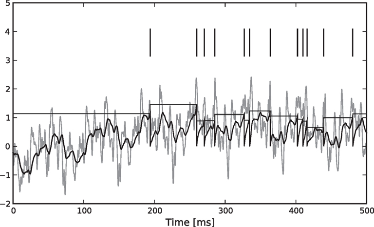
Figure 1. Illustration of the encoding process. We simulated a leaky (τ = 10) integrate-and-fire neuron with threshold noise (mean 1.0, variance 0.05). The input is a pink noise process consisting of 80 basis functions, 40 sine and 40 cosine, frequencies equally spaced between 1 and 500 Hz. The stimulus is plotted in shaded gray, the membrane potential in black. The threshold is drawn randomly according to a gamma distribution every time a spike (vertical lines) is fired.
In the previous section, we have seen that the encoding process can be described by a conditional distribution p(r |s), the probability of observing a neural response r, given that a stimulus s was presented. For the task of decoding, an important conceptual distinction can be made between point estimation and probabilistic inference. The latter consists of inferring the full posterior distribution p(s |r): the probability of stimulus s, given that we observed a specific neural response r. Point estimation in contrast requires to make a decision for one particular stimulus as a best guess. Typical point estimates are the posterior mean 𝔼[s |r] or the stimulus s* for which the posterior distribution takes its maximum (maximum a posteriori, MAP). These choices are optimal for different loss functions. A loss function specifies the ‘cost’ of guessing stimulus  if the true stimulus was s. The posterior mean is optimal for the squared error loss
  , whereas the MAP is optimal under the 0/1 loss. Although the 0/1 loss, which has a constant loss for arbitrarily small errors, is an arguably unnatural choice for continuous stimuli, MAP decoding is still popular and often performs well also with respect to other loss functions. Further, the posterior mean together with the posterior variance can also be regarded as a Gaussian approximation to the full posterior distribution.
if the true stimulus was s. The posterior mean is optimal for the squared error loss , whereas the MAP is optimal under the 0/1 loss. Although the 0/1 loss, which has a constant loss for arbitrarily small errors, is an arguably unnatural choice for continuous stimuli, MAP decoding is still popular and often performs well also with respect to other loss functions. Further, the posterior mean together with the posterior variance can also be regarded as a Gaussian approximation to the full posterior distribution.In the following we will start from the noiseless case, re-deriving the pseudo-inverse decoding scheme that has been presented before by (Seydnejad and Kitney, 2001
). We show that when introducing noise, the pseudo-inverse can still be seen as an approximate decoding rule, but suffers from an asymptotic bias. In order to cope with this problem, we derive a bias-reduced version as well, which canbe applied in an iterative ‘spike-by-spike’ fashion.
Noiseless Case
In the noiseless case, the problem of inverting the mapping from stimulus to spike-times can be interpreted as a linear mapping (see Seydnejad and Kitney, 2001
; Pillow and Simoncelli, 2002
; Arcas and Fairhall, 2003
). Roughly speaking, each interspike interval defines one linear constraint on the set of possible stimuli that could have evoked the observed spike response. The evolution of the membrane potential during an interspike interval is obtained via Eq. 2. As the spike times correspond to threshold crossings of the membrane, we know that the membrane potential hits the threshold θ at time tk:
If we represent the stimulus in terms of a linear superposition of basis functions (see Encoding), we can address the decoding problem within the framework of finding a linear inverse mapping. Decoding of the stimulus signal I(t) is equivalent to inferring the coefficients ci from the observed spike trains. Every interspike interval imposes a linear constraint on the coefficients ci.

where the components of y are defined as in Eq. 7. Note that Eq. 10 is a necessary condition for the coefficients. The unknown coefficients c can be uniquely determined if the number of linearly independent constraints is equal to or larger than the number of unknown coefficients (see also Figure 2
). We can summarize the constraints compactly in a linear equation:
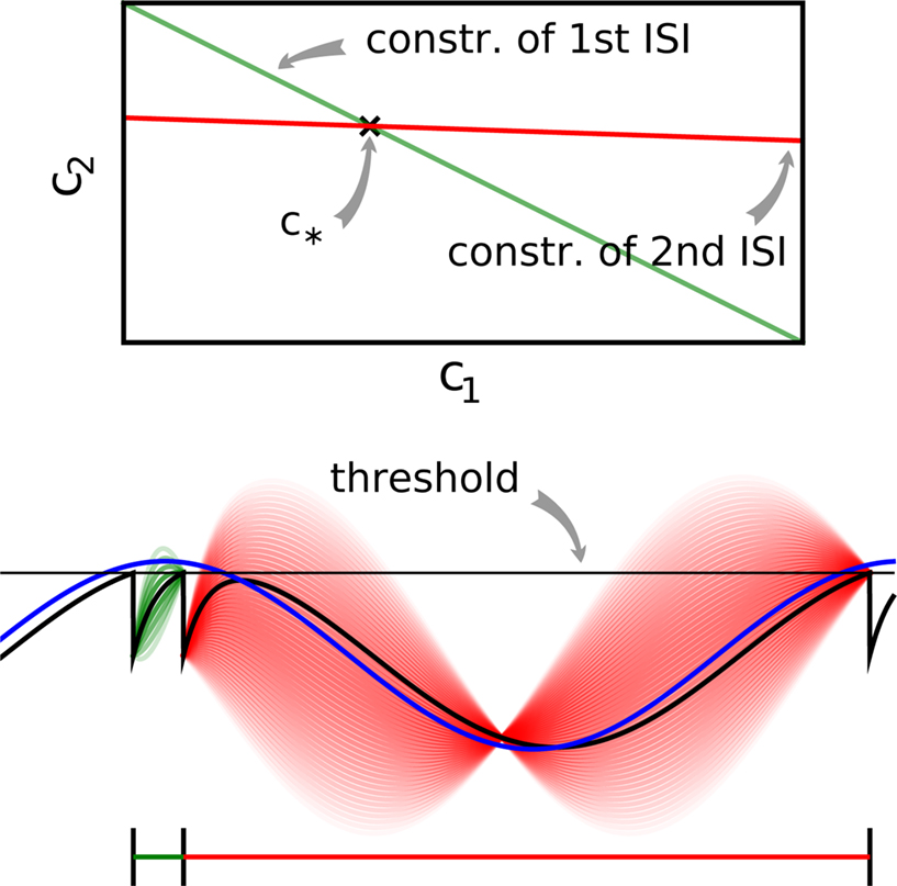
Figure 2. Example of noiseless decoding for a two dimensional stimulus and its limitations. The inset illustrates the linear constraints that the first and the second interspike interval pose on the two coefficients c1 and c2. The driving stimulus is plotted in blue. Vertical bars at the bottom indicate the three observed spike times corresponding to threshold crossings of the membrane potential (solid black). Possible membrane potential trajectories, which obey the linear constraints are plotted in shaded green and red respectively, darker ones have smaller norm. As can be seen the linear constraints only reflect that the membrane potential has to be at zero at the beginning of an interspike interval and at the threshold at the end of it. They do not reflect that the membrane potential has to stay below threshold between spike times. Parameters are: τ = 1 ms, frequency for sine and cosine basis functions: 32 Hz.
In general, a solution to this equation can be found by using the Moore–Penrose pseudo-inverse (Penrose, 1955
):

The pseudo-inverse is well defined even if the matrix L is not square or is rank-deficient. If the number of interspike intervals exceeds the number of coeffidown the posterior exactly:cients, the pseudo-inverse is given by:

Decoding in the Presence of Noise
One dimensional stimulus: exact inference
We start with a simple case in which exact inference is possible: the stimulus consists of a constant (one dimensional) input c, i.e. fi ≡ 1. In this situation, we can write down the likelihood exactly. For the observations we have:
In this case, we do not have to account for the sub-threshold condition as the evolution of the membrane-potential since the last spike is a monotonic function and therefore there is only one possibility to be at the threshold for a given stimulus at a specific time. In particular, if the threshold is Gamma distributed (as assumed in ‘Introduction’), we see that yk|c is also Gamma distributed with parameters α, β/c. For now we choose c to be Gamma distributed as well (say with parameters α0, β0). This choice deviates from the choice in the Section ‘Encoding’, but for this choice, we can write down the posterior exactly:
Having the posterior in closed form we can calculate the posterior mean as well as the point of maximal posterior probability exactly. Thus, we have in the special case of a constant one-dimensional input a reference for later use (see also Figure 3
).
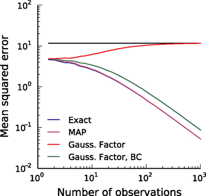
Figure 3. Comparison of the mean squared error (MSE) for different reconstruction methods in the case of a one dimensional stimulus. The best possible estimate is the true posterior mean (exact, blue). The error of the maximum a posteriori (MAP) estimator (magenta) is nearly the same as the error of the exact posterior mean and therefore cannot be distinguished from the exact one. The red line shows the error of the Moore–Penrose pseudo-inverse and the horizontal line indicates its asymptotic bias. The Moore–Penrose pseudo-inverse is called Gaussian Factor approximation (see Encoding). The bias corrected (BC) version of the Gaussian approximation (green) is explained later and here included for completeness (see Decoding). Parameters were: αprior = 20, βprior = 0.5, αθ = 2, βθ = 0.5.
Gaussian factor approximation
The pseudo-inverse solution of the Section ‘Introduction’ has also a probabilistic interpretation in linear Gaussian models (see also Bishop, 2006
): In this setting, it can be interpreted as the posterior mean estimate for data with a Gaussian distribution. In particular, if (for the moment) we assume that the linear functionals  are observed and that
  is Gaussian distributed around the mean of the threshold θ with a constant variance
  the posterior mean of the coefficients c would be the same as the pseudo-inverse described above. However, this setting is not directly applicable to the context of decoding a stimulus from spike times of LIFs: In a linear Gaussian model, the observed functionals
  would not be allowed to depend on either c or θ, but they do here. This is most easily explained for a one-dimensional stimulus: We have that θ = cy, and therefore y = θ/c. This can be highly non-Gaussian even if the distribution of θ and c are Gaussian
1
. We now derive a probabilistic decoding rule which is analogous to the pseudo-inverse used in the noiseless case. Each observation defines a linear constraint:
would not be allowed to depend on either c or θ, but they do here. This is most easily explained for a one-dimensional stimulus: We have that θ = cy, and therefore y = θ/c. This can be highly non-Gaussian even if the distribution of θ and c are Gaussian
1
. We now derive a probabilistic decoding rule which is analogous to the pseudo-inverse used in the noiseless case. Each observation defines a linear constraint:
are observed and that is Gaussian distributed around the mean of the threshold θ with a constant variance the posterior mean of the coefficients c would be the same as the pseudo-inverse described above. However, this setting is not directly applicable to the context of decoding a stimulus from spike times of LIFs: In a linear Gaussian model, the observed functionals would not be allowed to depend on either c or θ, but they do here. This is most easily explained for a one-dimensional stimulus: We have that θ = cy, and therefore y = θ/c. This can be highly non-Gaussian even if the distribution of θ and c are Gaussian
1
. We now derive a probabilistic decoding rule which is analogous to the pseudo-inverse used in the noiseless case. Each observation defines a linear constraint:
We can approximate the distribution of the threshold by a Gaussian term. Each linear constraint defines one factor of the likelihood. That is, pθ in Eq. 3 is replaced with a Gaussian term of the form:
where  is the variance of the threshold distribution. Additionally, we have replaced θ by its mean μθ, because we are not observing θ but tk. Each of these factors peaks at
  , therefore reflecting the linear constraint. Replacing every term in the likelihood by its corresponding Gaussian approximation and including one Gaussian factor for the prior
  , the posterior is approximated by a Gaussian with the following moments:
is the variance of the threshold distribution. Additionally, we have replaced θ by its mean μθ, because we are not observing θ but tk. Each of these factors peaks at , therefore reflecting the linear constraint. Replacing every term in the likelihood by its corresponding Gaussian approximation and including one Gaussian factor for the prior , the posterior is approximated by a Gaussian with the following moments:
In (16) and (17), we have abbreviated  . In addition to the pseudo-inverse (Eq. 12), this approximation takes the prior distribution over stimuli into account, specified by the mean μc and covariance Σc of the coefficients c. This can be seen by
  setting i.e. by using an uninformative prior. Then the mean of this approximation μp is exactly the pseudo-inverse of Eq. 12. Our approach of replacing likelihood factors by Gaussians is similar to the extended Kalman filter, where the dynamics is linearized and therefore results in a Gaussian update for the hidden states. However, it is known that this approximation can be biased (see Julier and Uhlmann, 1997
; Minka, 2001
). Similarly, in our case, the mean of this approximation also does not converge to the true coefficient values for increasing number of observed spikes, as shown in Figure 3
. Fortunately, under some simplifying assumptions, this bias can be calculated and therefore can be significantly reduced as will be shown in the following section.
setting i.e. by using an uninformative prior. Then the mean of this approximation μp is exactly the pseudo-inverse of Eq. 12. Our approach of replacing likelihood factors by Gaussians is similar to the extended Kalman filter, where the dynamics is linearized and therefore results in a Gaussian update for the hidden states. However, it is known that this approximation can be biased (see Julier and Uhlmann, 1997
; Minka, 2001
). Similarly, in our case, the mean of this approximation also does not converge to the true coefficient values for increasing number of observed spikes, as shown in Figure 3
. Fortunately, under some simplifying assumptions, this bias can be calculated and therefore can be significantly reduced as will be shown in the following section.
. In addition to the pseudo-inverse (Eq. 12), this approximation takes the prior distribution over stimuli into account, specified by the mean μc and covariance Σc of the coefficients c. This can be seen by setting i.e. by using an uninformative prior. Then the mean of this approximation μp is exactly the pseudo-inverse of Eq. 12. Our approach of replacing likelihood factors by Gaussians is similar to the extended Kalman filter, where the dynamics is linearized and therefore results in a Gaussian update for the hidden states. However, it is known that this approximation can be biased (see Julier and Uhlmann, 1997
; Minka, 2001
). Similarly, in our case, the mean of this approximation also does not converge to the true coefficient values for increasing number of observed spikes, as shown in Figure 3
. Fortunately, under some simplifying assumptions, this bias can be calculated and therefore can be significantly reduced as will be shown in the following section.Bias reduction of the gaussian factor approximation
In this section we calculate the asymptotic length bias for the approximate posterior mean of Eq. 16, assuming a correct orientation of the coefficient vector. By fixing a stimulus, i.e. c, we define the average over all resulting interspike intervals 𝔼[yk]: = μy and Cov[yk]: = Σy. We then find asymptotically for n >> 1 and for a fixed c:
Note that we do not know the distribution of the yk and that this distribution depends on the distribution of the threshold as well as the choice of basis functions. However, the proportion of y in the direction of c is on average of magnitude μθ and the variance along c on the other hand is  Orthogonal to c, we assume, that y has zero mean and finite variance. This assumption is justified in the one-dimensional case, because there is simply no orthogonal direction. Empirically, it turns out to reduce the amount of bias substantially; see Figure 6
.
Orthogonal to c, we assume, that y has zero mean and finite variance. This assumption is justified in the one-dimensional case, because there is simply no orthogonal direction. Empirically, it turns out to reduce the amount of bias substantially; see Figure 6
.
Orthogonal to c, we assume, that y has zero mean and finite variance. This assumption is justified in the one-dimensional case, because there is simply no orthogonal direction. Empirically, it turns out to reduce the amount of bias substantially; see Figure 6
.Therefore, we can rewrite
where
with
Here, c⊥ denotes the basis for the space orthogonal to c and  are the variances in the direction of the basis vectors of c⊥ which are not important for the calculation of the bias. Wecan now compute the asymptotic posterior mean:
are the variances in the direction of the basis vectors of c⊥ which are not important for the calculation of the bias. Wecan now compute the asymptotic posterior mean:
We obtain (21) from (20) by using the Woodbury matrix identity. By definition of U, all directions orthogonal to c cancel out and Eq. 22 follows. Equation 22 shows that (asymptotically) the norm of the posterior mean approximation is biased. The direction, however, is correct. Therefore, the Moore–Penrose pseudo-inverse is unbiased only in the noiseless case when  In the noisy case, however, we can divide the mean by its asymptotic bias in order to obtain an unbiased estimator for the coefficients. To improve the estimator also in the regime of few observations, we divide only the likelihood part
  by the asymptotic bias. Therefore we have for the bias-reduced posterior mean:
In the noisy case, however, we can divide the mean by its asymptotic bias in order to obtain an unbiased estimator for the coefficients. To improve the estimator also in the regime of few observations, we divide only the likelihood part by the asymptotic bias. Therefore we have for the bias-reduced posterior mean:
This bias-reduced version of the Moore–Penrose inverse is also plotted in Figure 3
, which gives an improved estimate also for a small number of observations. The presented bias-reduced Gaussian approximation can also be rewritten into an online algorithm. The update equations to incorporate one additional observation yk in the current posterior are given by:
Together with Eq. 23 we thus obtain a bias-reduced on-line estimator which allows one to recursively improve the stimulus reconstruction on a spike-by-spike basis:
We can now compare how well the different approximations perform compared to the exact solution in the one-dimensional case (see Introduction). In Figure 3
the mean squared error is shown as function of the number of observed interspike intervals. Plotted are the error of the MAP estimator (magenta), the exact minimum mean squared error (blue), the Gaussian-Factor approximation, which is the equivalent to the Moore–Penrose pseudo-inverse (red) and the bias reduced Gaussian-Factor approximation (green). Importantly, the solution obtained by the Moore–Penrose pseudo-inverse does not converge to the true solution, but hasa strong bias. This bias can lead to a solution which is actually worse than the prior solution. Unfortunately, we do not have access to the exact posterior in general, especially in higher dimensions. Therefore, we need approximation schemes which are generally applicable in the general case, but which perform better than the Moore–Penrose pseudo-inverse.
Two-Dimensional Case
In the section ‘Introduction’, we investigated the accuracy of the different reconstruction schemes in the one-dimensional case. If the stimulus is two- or higher-dimensional, the observation of a single spike does not give us full rank information about the stimulus. In the case of a two-dimensional stimulus, three types of scenarios can occur after one interspike interval has been observed:
1. The observation of an interspike interval only leads to one important constraint on the coefficients of the basis functions, namely that the membrane potential has to be at the threshold at the time of a spike. For example, if the observed interspike interval is relatively small, solutions which cross the threshold twice or hit the threshold from above, are very unlikely under the prior distribution. Therefore, to stay below threshold, one can neglect constraints other than being atthe threshold at the time of the observed spike, see also Figure 2
. In this situation, all approximations should be almost equally good as they all account for this type of constraint.
2. If the interspike interval is longer, we might get another important constraint for the posterior, namely by requiring that the threshold is hit from below, not from above. This possibility is ruled out by the Jacobian term of the pseudo-likelihood (Eq. 32). Therefore the MAP estimate should be closer to the true posterior mean than the Gaussian or pseudo-inverse approximation, which does not satisfy this constraint. Here, crossing the threshold twice before hitting it again from below is still very unlikely according to the prior and therefore we do not get an effective restriction for the posterior by ruling out all these solutions which cross the threshold twice.
3. If the interspike interval is sufficiently long, both types of violations of crossing the threshold between spike times are probable according to the prior. Some possible stimuli might exist for which the membrane potential would cross the threshold twice before reaching the threshold again at the time of the observed spike. These stimuli are neither ruled out by the pseudo-likelihood nor by the Gaussian approximation. Therefore, both approximations can result in quite poor estimates of the true posterior mean.
To illustrate the three scenarios, we simulated a single neuron with a stimulus consisting of two basis functions, one sine and one cosine function. We obtained an approximation to the true posterior after single observations by rejection sampling. This true posterior reflects all of the constraints mentioned above. As can be seen in Figure 4
, indeed three types of situations can be observed.
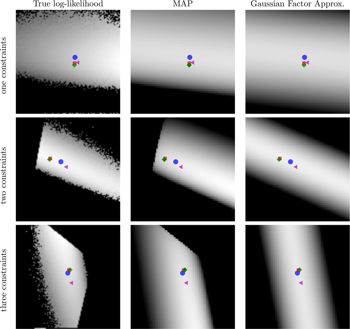
Figure 4. Log-likelihood approximations in two dimensions for three different cases of observations and different approximations to the posterior. The first column is the true log-likelihood, the second is the approximate log-likelihood obtained by Eq. 43 and the third column is the Gaussian Factor approximation. The true log-likelihood is not available in higher dimensions and is plotted here for comparison and as a reference. It is obtained via rejection sampling. Point estimates are: true posterior mean ( ), MAP (
 ), Gaussian Factor mean (
 ) and the bias reduced version (
 ). For each point estimate a Gaussian prior with unit isotropic covariance was chosen. Each subplot shows the log-likelihood (or its approximation) after one interspike interval is observed. The x and y axes indicate the two dimensions of the stimulus coefficients. Each row corresponds to a different scenario with different numbers of effective constraints for the posterior. If only one constraint is active (first row) the true posterior does not differ much from the other approximations, and therefore the point estimates perform all almost equally well. If two constraints are active (the threshold has to be reached from below and the membrane potential has to be at the threshold at the time of a spike) the MAP performs better than the Gaussian Factor approximation. If three constraints are active, the MAP reflects two of the three constraints and therefore is slightly shifted. As one observation is far away from the asymptotic regime, the Gaussian Factor approximation and its bias reduced version do not differ much.
), MAP (), Gaussian Factor mean () and the bias reduced version (). For each point estimate a Gaussian prior with unit isotropic covariance was chosen. Each subplot shows the log-likelihood (or its approximation) after one interspike interval is observed. The x and y axes indicate the two dimensions of the stimulus coefficients. Each row corresponds to a different scenario with different numbers of effective constraints for the posterior. If only one constraint is active (first row) the true posterior does not differ much from the other approximations, and therefore the point estimates perform all almost equally well. If two constraints are active (the threshold has to be reached from below and the membrane potential has to be at the threshold at the time of a spike) the MAP performs better than the Gaussian Factor approximation. If three constraints are active, the MAP reflects two of the three constraints and therefore is slightly shifted. As one observation is far away from the asymptotic regime, the Gaussian Factor approximation and its bias reduced version do not differ much.In the following, we will discuss the relationship between our decoding rule and previously proposed decoding algorithms. In particular, we compare our decoders with an optimal linear decoder, as well as with a Maximum-a-Posteriori decoder (MAP) based on the approximate likelihood.
Relationship with Linear decoder
Bialek et al. popularized a linear decoder for reconstructing the stimulus from a spike train (Bialek et al., 1991
; Rieke et al., 1997
). Here the spike train  is convolved with an acausal linear filter K in order to obtain an estimate of the stimulus:
is convolved with an acausal linear filter K in order to obtain an estimate of the stimulus:
The filter can be calculated by (see Rieke et al., 1997
):
where ℱ is the Fourier transform. The average is taken over the joint distribution of stimuli and spike times, which can be done via sampling. Additionally, the stimuli we used are composed by a superposition of sine and cosine functions with discrete frequencies, which we write here as complex functions  . Hence, the linear filter has also only non-vanishing power in those frequencies which are present in the stimulus.
. Hence, the linear filter has also only non-vanishing power in those frequencies which are present in the stimulus.In the noiseless case, the Pseudo-Inverse decoder can be interpreted as a linear filter, but one that depends on the particular spike train observed, as we will show in the following. To this end, we replace the stimulus ensemble used to calculate the linear filter with a single stimulus consisting of the stimulus reconstructed by the Pseudo-Inverse. That is, we replace  by
by  see Eq. 12. If we furtherassume that there is no neuronal noise, we can neglect the expectation in the definition of the linear filter (Eq. 12), and define a linear filter Kp corresponding to the Pseudo-Inverse:
by see Eq. 12. If we furtherassume that there is no neuronal noise, we can neglect the expectation in the definition of the linear filter (Eq. 12), and define a linear filter Kp corresponding to the Pseudo-Inverse:
Although this equivalence is only valid in the noiseless case, we can use Eq. 29 to illustrate the decoding performed by the Pseudo-Inverse. The linear filters we obtain for this decoder is different for different spike trains, reflecting the increased flexibility of the Pseudo-Inverse compared to the optimal linear predictor. The different reconstructions and associated filters are illustrated in Figure 5
.
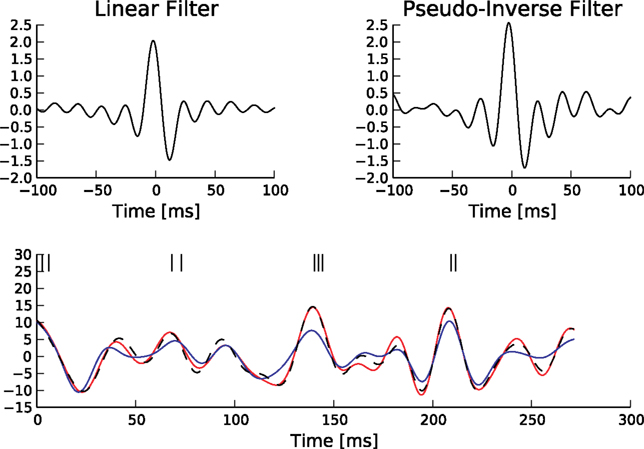
Figure 5. Comparison of the linear decoder and the Gaussian factor approximation. Upper left: Linear filter obtained via Eq. 28. Upper right: Average linear filter for the Pseudo-Inverse or Gaussian factor approximation, see Eq. 29. Bottom: Example of a decoded stimulus for a given spike train by two decoding schemes. The true stimulus is plotted in dashed black, the Gaussian factor reconstruction in red and the linear decoder reconstruction is plotted in blue. Shown are a window of the first 10 out of 100 spikes. The stimulus consisted of 20 sine and 20 cosine functions with frequencies between 10 and 50 Hz. Spikes are generated with a leaky integrator withtime constant τ = 25 ms. The noise is relatively low:  The squared errors for the trial here are: 3.27 for the linear decoder and 2.11 for the pseudo inverse.
The squared errors for the trial here are: 3.27 for the linear decoder and 2.11 for the pseudo inverse.MAP and laplace approximation
By inspecting the approximate likelihood (see Eq. 8) we see that the model is a generalized linear model. In this sense it is very similar to the soft-threshold noise model (Jolivet et al., 2006
; Paninski et al., 2007
). However, the threshold noise there is Poisson-like, whereas here it is Gamma distributed. Further, the soft-threshold likelihood does not account for the fact that the threshold has to be reached from below. By ensuring that the Jacobian of the change of variables in Eq. 3 is positive, however, we can take this constraint into account. One approach for getting a possibly better point estimate is to find the maximum of the approximate posterior density (MAP). To compute this posterior density, we have to multiply Eq. 3 by the prior density (which is Gaussian in our case). In this model, the MAP cannot be determined in closed form, but we may apply gradient ascent in order to find it numerically. If both likelihood and prior are log-concave, which is true for the approximate likelihood and the Gaussian prior used here, the posterior is unimodal (see Paninski et al., 2004
). Hence, finding the MAP point is a convex problem. The gradient and the Hessian of the log posterior are straightforward to compute. For the sake of clarity, we only write down the gradient and the Hessian for one spike time tk in the sum of Eq. 8:
Here, f(tk) is the vector consisting of all basis functions evaluated at the spike time tk. The Hessian is given by:
Applying a gradient ascent scheme yields a point estimate that respects the constraint that the membrane potential crosses the threshold from below. Nevertheless, it does not take into account the sub-threshold condition between spike times: The solution we get might correspond to a membrane potential that crosses the threshold twice before it hits it again from below. Therefore this point estimate suffers from the same source of bias as the Gaussian factor approximation.
This point estimate can be extended to give an approximation of the uncertainty as well by expanding the posterior to second order around the MAP point. The posterior we are using here is the likelihood (Eq. 3) times a prior term p(c):
which itself is an approximation (see Introduction). Unfortunately, computing the normalization constant for this distribution with respect to c is not tractable. We therefore approximate the posterior by a second-order expansion. In other words, the posterior distribution is approximated by a multivariate Gaussian, where the mean of the Gaussian is taken to be the MAP, and the covariance is found by looking at the second-order derivatives of the log-posterior at the MAP:
The MAP and the Hessian are calculated by Eqs 30 and 31. This yields a Gaussian approximation known as the Laplace approximation (MacKay, 2003
; Rasmussen and Williams, 2006
; Paninski et al., 2007
; Cunningham et al., 2008
).
In this section, we present the results of three different simulations which highlight different aspects of neural population coding of time-varying stimuli with integrate and fire neurons. As a general framework, we first specify a generative model for the stimulus signal  and then we specify a mapping
  , which can be interpreted as the encoding strategy of the neural population. The dimension of
  can be different from the number of spatial stimulus components m. Each Ii(t) represents one neuron within a population of n neurons. Each spatial component xl(t),l = 1,…,m is represented with a superposition of temporal basis functions fk(t),k = 1,…, M. In the first simulation we have n = m = 1, M = 80. In the second and third simulation
  . In the last simulation we study the encoding of an amplitude and phase variable with
  .
.
and then we specify a mapping , which can be interpreted as the encoding strategy of the neural population. The dimension of can be different from the number of spatial stimulus components m. Each Ii(t) represents one neuron within a population of n neurons. Each spatial component xl(t),l = 1,…,m is represented with a superposition of temporal basis functions fk(t),k = 1,…, M. In the first simulation we have n = m = 1, M = 80. In the second and third simulation . In the last simulation we study the encoding of an amplitude and phase variable with .Simulation 1: One Neuron, One Component, Many Temporal Dimensions
In order to evaluate the accuracy of our Gaussian Factor approximation to the posterior when the stimulus has several temporal dimensions (not to be confused with spatial dimensions m), we analyzed the decoding performance as a function of increasing number of observations. To this end, we simulated a neuron with a stimulus consisting of a random superposition of 40 sine and 40 cosine functions with equally spaced frequencies between 10 and 50 Hz. In each trial the neuron was simulated until 104 spikes were accumulated. We calculated the mean squared error over 100 repetitions. Interspike intervals taken into account for reconstruction were randomly selected from the whole time interval of the simulation.
In Figure 6
we see that the simple Gaussian approximation (Gaussian Factor, red, dashed) is indeed biased and the bias is larger for larger noise levels. In the limit of no noise we expect a sharp drop off for the number of spikes equal to the number of dimensions for the stimulus. This is weakened in the presence of noise. For comparison, we also plot the asymptotic error of the Gaussian Factor approximation as derived analytically in the Section ‘Decoding’. Additionally the mean squared errors are plotted for the linear decoder (see Introduction) and the bias-reduced version of the Gaussian approximation. The mean squared error for the MAP was obtained by gradient ascent (see Introduction). In order to start with a feasible solution, we initialized the optimizer with the true stimulus coefficients, turning the obtained solution in an optimistic estimate of the actual MAP.
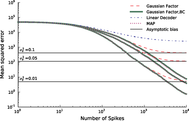
Figure 6. Mean squared error (MSE) as a function of the number of spikes used for the different decoding schemes. The stimulus consists of a superpostion of 40 sine and 40 cosine functions of discrete frequencies equally spaced between 10 and 50 Hz. The time constant of the neuron used for decoding is τ = 25 ms. The MSE is calculated as the average over 100 repetitions for three different noise levels. Horizontal lines indicate the asymptotic bias for the different noise levels. The prior was an isotropic Gaussian with zero mean and covariance matrix 𝟙 · 25.
Simulation 2: Many Neurons, Many Temporal Dimensions
In this simulation, a population of n = 30 neurons with different receptive fields were all driven by the same stimulus, which consisted of a superposition of 20 sine and 20 cosine functions  The frequencies
  were equally spaced between 1 and 100 Hz, and the coefficients
  were drawn independently from a Gaussian distribution with unit variance.
The frequencies were equally spaced between 1 and 100 Hz, and the coefficients were drawn independently from a Gaussian distribution with unit variance.Incorporating a receptive field ri(t) for neuron i in our model can easily be done by pre-filtering the stimulus with the corresponding receptive field:
Because of the linearity of the convolution, the decoding algorithms stay the same with the exception that the basis functions fk(s) are replaced by  . The receptive fields ri(t) of each neuron were chosen to be a gamma tone:
. The receptive fields ri(t) of each neuron were chosen to be a gamma tone:
All parameters except the frequency f were fixed (a = 0.01, b = 0.01  n = 2, ϕ = 0). The frequencies of each receptive field were drawn from a uniform distribution ranging between 1 and 100 Hz. The resulting receptive fields are shown in Figure 7
(left). The stimulus and its reconstruction based on the spike times of this population are shown in Figure 7
(right). The uncertainty is smaller within periods of higher firing rates, yet to a smaller extent than in the next setting (see Figure 9
), because here the receptive fields have a larger temporal extent.
n = 2, ϕ = 0). The frequencies of each receptive field were drawn from a uniform distribution ranging between 1 and 100 Hz. The resulting receptive fields are shown in Figure 7
(left). The stimulus and its reconstruction based on the spike times of this population are shown in Figure 7
(right). The uncertainty is smaller within periods of higher firing rates, yet to a smaller extent than in the next setting (see Figure 9
), because here the receptive fields have a larger temporal extent.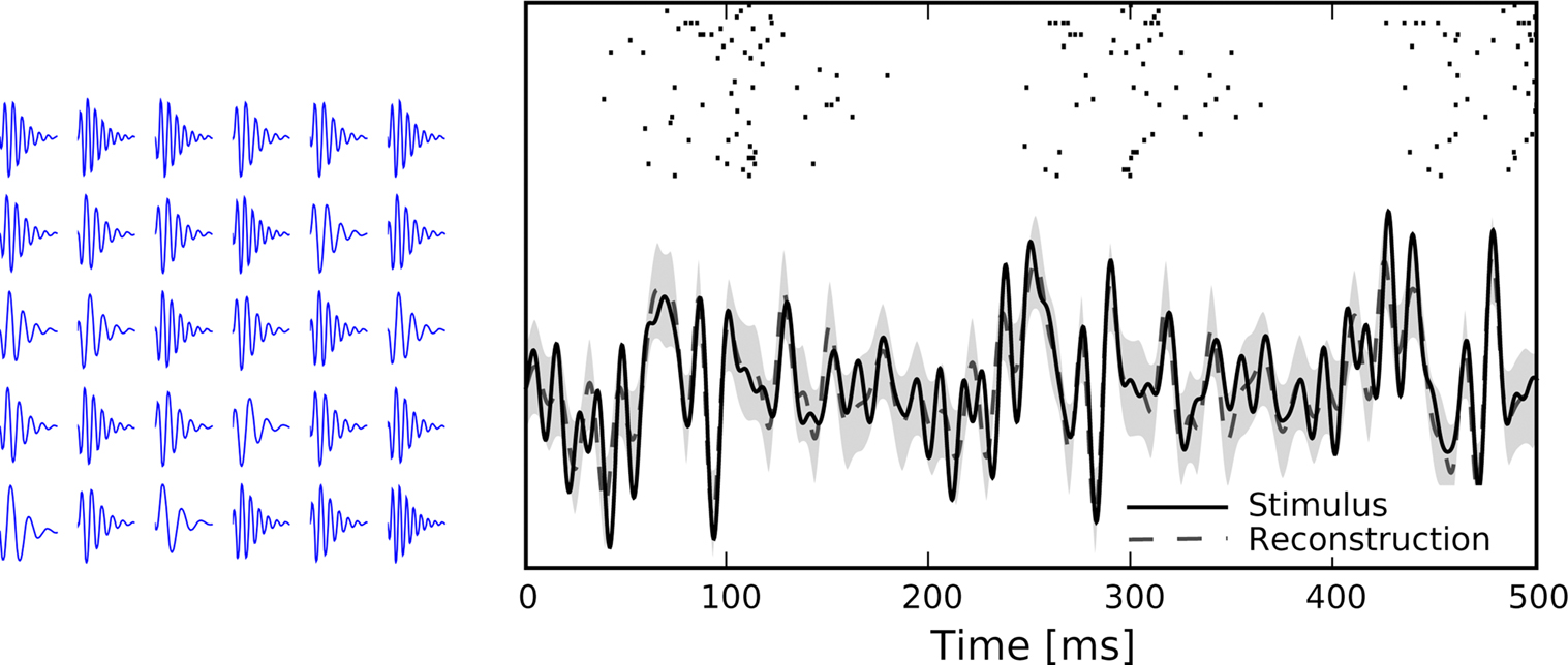
Figure 7. Left: Receptive fields of the population, each is a gamma tone with a different frequency, randomly drawn from a uniform distribution between 1 and 100 Hz. Right: A time varying stimulus consisting of a superposition of 20 sine and 20 cosine functions is decoded from spike trains of a population of 30 neurons, each having a noise level of σθ = 0.05.
Simulation 3: Heterogeneity
Every new spike contributes new information about the stimulus, and leads to a reduction in reconstruction error. However, if the resulting linear constraints are correlated, the reduction can be arbitrarily small. This problem can become particularly severe for interspike intervals observed at different neurons. For example, if the parameters of different neurons (e.g. the receptive fields) are the same, spikes of different neurons tend to synchronize, even in the presence of threshold noise. This leads to similar interspike intervals, and thus to highly correlated linear constraints. In this case, the information conveyed by different neurons can be redundant and be of limited use for decoding.
It is plausible that efficient population codes should have heterogeneity in their receptive field properties, to ensure that different properties of the stimulus are sampled by the population. In our setting, diversity in receptive field parameters would ensure that the constraints are less correlated and that the reconstruction error does not saturate with increasing numbers of neurons. As a result, we expect to get a better reconstruction if we have a larger diversity within the encoding population.
In this simulation, we extend the previous example by systematically varying the degree of similarity in the receptive field properties among the different neurons. To construct heterogeneous populations with different degrees of diversity we sampled the center frequencies of the receptive field (gamma tone) of each neuron from a uniform distribution within a frequency interval centered at 50 Hz (the center frequency of the stimulus used). The degree of diversity was then measured by the length of thisinterval, from 0 to 25 Hz. Figure 8
shows the mean squared error as a function of number of neurons as well as the diversity within the receptive fields. From this plot one can see that the rate with which the error drops with increasing number of neurons strongly depends on the degree of diversity. This result confirms the general idea of redundancy reduction as an efficient coding strategy.
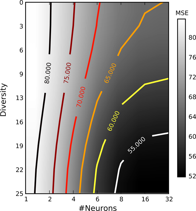
Figure 8. Mean squared error as a function of the number of neurons and their diversity within their receptive fields. Diversity is measured by the width of the uniform distribution from which frequencies for the gamma tone receptive fields were drawn. The average is taken over ≥25 repetitions. All other parameters were as in the previous section.
Simulation 4: Encoding of Amplitude and Phase Variables
In this simulation we consider the case of decoding a two-dimensional, time-varying stimulus signal. In particular, we want to illustrate how the encoding of angular variables can be addressed in this framework, as the neural representation of edge orientations or motion directions are frequently studied in neuroscience. Therefore, we use the nonlinear polar coordinate transform to obtain an amplitude and phase variable  as our stimulus signal. For simplicity, we consider the case where this signal is encoded by two neurons with identical temporal receptive field properties but with 90° difference in the preferred stimulus angle. Specifically, the encoding model of the two neurons is given by:
as our stimulus signal. For simplicity, we consider the case where this signal is encoded by two neurons with identical temporal receptive field properties but with 90° difference in the preferred stimulus angle. Specifically, the encoding model of the two neurons is given by:
As temporal basis functions we picked 20 sine and cosine basis functions with discrete equally spaced frequencies between 1 and 10 Hz. The corresponding coefficients ck were drawn independently from a Gaussian distribution with variance
2
σ2 = 0.06. The neurons were simulated according to Eq. 1, with parameters  As can be seen from Figure 9
, the two dimensional signal (bottom two panels) can be reconstructed best in those time intervals which contains spikes (vertical black lines). The reconstruction and uncertainty (obtained via sampling) are transformed into phase and amplitude in the top two panels.
As can be seen from Figure 9
, the two dimensional signal (bottom two panels) can be reconstructed best in those time intervals which contains spikes (vertical black lines). The reconstruction and uncertainty (obtained via sampling) are transformed into phase and amplitude in the top two panels.
As can be seen from Figure 9
, the two dimensional signal (bottom two panels) can be reconstructed best in those time intervals which contains spikes (vertical black lines). The reconstruction and uncertainty (obtained via sampling) are transformed into phase and amplitude in the top two panels.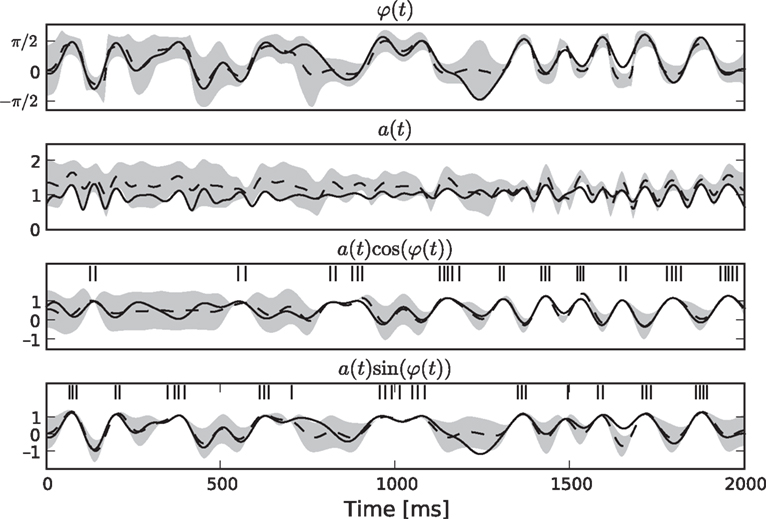
Figure 9. Decoding of an angular variable. Two neurons were stimulated with a(t)sinφ(t) and a(t)cosφ(t), respectively (two bottom panels). Each of those signals was represented by a superposition of 20 sine and 20 cosine functions. From the reconstructed signal, the amplitude a(t) and the phase angle φ(t) were obtained by taking the Euclidean norm and the arc-tangent, respectively. The reconstruction (dashed) of the original stimulus (solid) was obtained by using the Gaussian approximation with bias correction. Confidence intervals, indicating one standard deviation of the posterior variance, are plotted in shaded gray. The confidence intervals of a(t) and φ(t) were calculated by drawing 5000 samples from the approximate posterior.
How to read out spatio-temporal spike patterns generated by populations of neurons is fundamental to the understanding of neural network computation. Most of the previous studies on population coding were limited to the static case where only spike countsfor a preset time window are considered. For the encoding of continuously varying signals, however, it is important to understand how the accuracy of population codes is affected by the dynamics of neural spike generation.
Here, we studied dynamic population codes with noisy leaky integrate-and-fire neurons. We presented an algorithm for Bayesian decoding similar to the one presented in Cunningham et al. (2008)
. In addition, we derived an approximate algorithm which yields a simple spike-by-spike update rule for recursively improving the stimulus reconstruction whenever a new spike is observed.
The decoding rules can also be applied for decoding the spike trains of populations of neurons, not just single neurons. Importantly, we do not have to assume that the neurons are uncoupled, i.e. conditionally independent given the stimulus. In particular, as we assume the encoding model to be known, we would also know the parameters describing the couplings between neurons. Then, the influence of one spike of a neuron on the membrane potential of any other neuron is just a known, given input and can be subtracted. Therefore, the same decoding framework can also be used for decoding coupled neurons.
The decoding rule is nonlinear and sensitive to the relative latencies between each spike and its predecessor in the population. However, it is not optimal as it does not use the information that the membrane potential stays below threshold between spikes. To incorporate this kind of knowledge one has to integrate the coefficient distribution over the linear halfspace confined by the threshold similar to the method described in Paninski et al. (2004
, 2007
) but with the additional complication that, the distribution is not Gaussian. Therefore, the optimal Bayesian decoding rule would be computationally much more expensive.
The main goal of this work was to derive a simple decoding rule that facilitates the analysis of neural encoding strategies such as efficient coding, unsupervised learning, or active sampling. Bayesian approaches are particularly useful for these problemsas they do not yield a point estimate only but also aim at estimating the posterior uncertainty over stimuli. Having access to this uncertainty allows one to optimize receptive field properties or other encoding parameters in order to minimize the reconstruction error or to maximize the mutual information between stimulus and neural population response. In this way it becomes possible to extend unsupervised learning models such as independent component analysis (Bell and Sejnowski, 1995
) or sparse coding (Olshausen and Field, 1996
) to the spatio-temporal domain with spiking neural representations. This seems highly desirable as comparisons between theoretically derived models and experimental measurements would thus become feasible.
Furthermore, animals do not receive the sensory input in a passive way but actively tune their sensory organs to acquire the most useful data, for example by changing gaze or by head movements. Such active sampling strategies are related to the theory of optimal design or active learning (Lewi et al., 2009
), where the next measurement is selected in order to minimize the current uncertainty about the signal of interest. Such active sampling strategies give rise to ‘saliency maps’, which encode the expected information gain from any particular stimulus.
Maximizing the mutual information between stimulus and neural response is equivalent to minimizing the posterior entropy. Because of the Gaussian approximation, this can be done in our model by performing a gradient descent on the log-determinant of the posterior covariance matrix. The gradient can be calculated from Eq. 17. However, the approximated posterior covariance derived in this paper might also be subject to a systematic deviation from the exact covariance matrix. Therefore, an important extension of the present work would be to correct for a bias in the approximate covariance estimate, too. In general the approximations considered in this paper usually tend to over-estimate the true underlying uncertainty, as they wrongly donot cut-off regions in the parameter space.
In this paper, we chose to represent the stimulus by a superposition of a finite set of basis functions as this has some practical advantages. Alternatively, it is also possible to start from a full Gaussian process as stimulus model and then derive a discretization for numerical evaluation. Analogous to the mean vector and covariance matrix of a finite-dimensional normal distribution, a Gaussian process prior over the stimulus is specified by the mean and covariance function of the process. For numerical evaluation it is necessary to choose a grid of time points yielding a finite dimensional normal distribution again. Note that for inference, integrals on the grid points have to be evaluated numerically and therefore a fine time resolution for the si should be chosen. Therefore, the computational load of decoding a discretized Gaussian process is considerably higher. For practical reasons, we can restrict the inference procedure to a time window around the current spikes, provided that the covariance function falls off quickly. In the non-leaky case with no receptive fields this is the same setting as in Cunningham et al. (2008)
.
The extension to the Gaussian process setting is conceptually important as it allows one to replace the somewhat artificial threshold noise model by membrane potential noise. The dynamics can then be described by a stochastic differential equation. Although the likelihood is much harder to calculate (Paninski et al., 2004
, 2007
), it still has the renewal property and therefore a similar approximation scheme might be applicable. However, it has the further complication, that the obtained likelihood is only for a given threshold and therefore the threshold has to be marginalized. We hope that more studies will be devoted to the problem of decoding time-varying stimuli from populations of spiking neurons in the future. In particular, it will be crucial to achieve a good trade-off between the basic dynamics of neural spike generation, the accuracy of posterior estimates and the computational complexity of the decoding algorithm.
The authors declare that the research was conducted in the absence of any commercial or financial relationships that could be construed as a potential conflict of interest.
This work is supported by the German Ministry of Education, Science, Research and Technology through the Bernstein award to Matthias Bethge (BMBF; FKZ: 01GQ0601). We would like to thank Ralf Häfner, Alexander Ecker and Philipp Berens for comments on the manuscript.
 and
and 